2. A first taste of AiiDA
Let’s start with a quick demo of how AiiDA can make your life easier as a computational scientist.
We’ll be using the verdi command-line interface,
which lets you manage your AiiDA installation, inspect the contents of your database, control running calculations and more.
As the first thing, open a terminal and type workon aiida to enter the “virtual environment” where AiiDA is installed.
You will know that you are in the virtual environment because each new line will start with (aiida), e.g.:
(aiida) max@qmobile:~$
Note that you will need to retype workon aiida every time you open a new terminal.
Here are some first tasks for you:
The
verdicommand supports tab-completion: In the terminal, typeverdi, followed by a space and press the ‘Tab’ key twice to show a list of all the available sub commands.For help on
verdior any of its subcommands, simply append the--help/-hflag:verdi -h
Note
This tutorial is a short crash course into AiiDA, focusing on Wannier90 as the code that AiiDA will run (via the aiida-wannier90 plugin).
Many more codes are supported by AiiDA (see full updated list of plugins on the AiiDA plugin registry). If you want to see a similar first-taste tutorial, but focused on Quantum ESPRESSO instead (using the aiida-quantumespresso plugin), you can check the “first-taste” page of the tutorial held in Ljubiana (2019).
2.1. Importing a crystal structure from a file
We will use a gallium arsenide (GaAs) primitive cell with 2 atoms in this first part of the tutorial.
We provide the crystal structure, in XSF format, here:
GaAs.xsf.
You can download the file in a folder in the virtual machine,
and then import it into AiiDA (via the ASE library)
using the following verdi command, run from a bash shell:
verdi data structure import ase GaAs.xsf
Each piece of data in AiiDA gets a PK number (a “primary key”)
that identifies it in your database.
This is printed out on the screen by the verdi data structure import command.
Mark it down, as we are going to use it in the next commands.
Note
In the next commands, replace the string <PK> with the appropriate PK number.
Let us first inspect the node you just created:
verdi node show <PK>
You will get in output some information on the node,
including its type (StructureData, the AiiDA data type for storing crystal
structures), a label and a description (empty for now, can be changed),
a creation time (ctime) and a last modification time (mtime),
the PK of the node and its UUID (universally unique identifier).
Note
When should I use the PK and when should I use the UUID?
A PK is a short integer identifying the node and therefore easy to remember. However, the same PK number (e.g., PK=10) might appear in two different databases referring to two completely different pieces of data.
A UUID is a hexadecimal string that might look like this:
d11a4829-3e19-4978-bfcf-c28ddeb0891e
A UUID has instead the nice feature to be globally unique: even if you export your data and a colleague imports it, the UUIDs will remain the same (while the PKs will typically be different).
Therefore, use the UUID to keep a long-term reference to a node. Feel free to use the PK for quick, everyday use (e.g. to inspect a node).
Note
All AiiDA commands accepting a PK can also accept a UUID. Check this by
trying the command above, this time with verdi node show <UUID>.
Note the following:
AiiDA does not require the full UUID, but just the first part of it, as long as only one node starts with the string you provide. E.g., in the example above, you could also say
verdi node show d11a4829-3e19. Most probably, instead,verdi node show d1will return an error, since you might have more than one node starting with the stringd1.By default, if you pass a valid integer, AiiDA will assume it is a PK; if at least one of the characters is not a digit, then AiiDA will assume it is (the first part of) a UUID.
How to solve the issue, then, when the first part of the UUID is composed only by digits (e.g. in
2495301c-dd00-42d6-92e4-1a8c171bbb4a)? As described above, usingverdi node show 24953would look for a node withPK=24953. As a solution, just add a dash, e.g.verdi node show 24953-so that AiiDA will consider this as the beginning of the UUID.Note that you can put the dash in any part of the string, and you don’t need to respect the typical UUID pattern with 8-4-4-4-12 characters per section: AiiDA will anyway first strip all dashes, and then put them back in the right place, so e.g.
verdi node show 24-95-3will give you the same result asverdi node show 24953-.
Try to use again
verdi node showon theStructureDatanode above, just with the first part of the UUID (that you got from the first call toverdi node showabove).
2.2. Running a job calculation
2.2.1. Introduction and importing existing simulations
In AiiDA, one very important type of calculation is called “calculation job” (whose logic is
implemented in a CalcJob python class, and that is stored upon execution using a CalcJobNode python class).
These calculations represent the execution
of an external code (e.g. Quantum ESPRESSO, Wannier90, …), very often on a different computer
than the one where AiiDA is installed.
The execution is automatically tracked by AiiDA (input creation, submission, waiting for the job scheduler,
file retrieval and parsing) and its inputs and outputs are connected to the CalcJobNode (representing
the execution) via INPUT and CREATE links.
In the following, we want to launch a CalcJob running a Wannier90 calculation.
Typically, before running a Wannier90 calculation, you need to obtain the .amn, .mmn, … files
from the interface to a first-principles code. In order to keep this tutorial focused on Wannier90, we have
already run that part with AiiDA (using Quantum ESPRESSO) and we will just import it into your database.
To achieve so, download this AiiDA export file:
example-gaas-wannier.aiida
and, once you have downloaded it in the current folder, run the following command in your bash shell:
verdi import example-gaas-wannier.aiida
This will import, in particular, the node with UUID 71155a0b-6cb9-4712-a043-dc4798ccfaaf,
that contains the .amn, .mmn, … files created by the pw2wannier90.x code of Quantum ESPRESSO.
Its provenance looks like the following figure (with some output nodes of the calculations not shown for clarity):

Fig. 2.10 Provenance graph for the FolderData node (71155a0b) that we have already run. At the top, we see the execution
of a get_primitive() calc function (described later in the appendix)
to obtain a primitive cell from a conventional cell.
The darker red rectangles represent the various calc jobs that we have run
for you, in particular:
the Quantum ESPRESSO SCF step (UUID
dcd4c286)the Quantum ESPRESSO NSCF step (UUID
be52abbf)the Wannier90 preprocess (
-pp) step (UUIDa95261e2)the Quantum ESPRESSO pw2wannier90 step (UUID
d34d62f9).
Exercise: To check that the import worked correctly, use verdi node show on the UUID of the FolderData
mentioned above to check that you indeed have the node in your database.
Exercise: FolderData is a type of node that stores an arbitrary set of files and folders in AiiDA.
Check the list of files included in it with the command verdi node repo ls 71155a0b, and check the content of
a given file (e.g. the aiida.mmn file) with verdi node repo cat 71155a0b aiida.mmn.
Exercise: In the figure above, verify that all calculations are connected between them via provenance links (through
some data node). Try to understand how, e.g., the NSCF calculation “restarts” from the SCF via a RemoteData node
(that represents a reference to the folder in the computational cluster where the SCF calculation was run), or how the
pw2wannier90 step uses as input both the RemoteData node of the NSCF and the .nnkp file generated by wannier90.x -pp.
2.2.2. Running Wannier90 with AiiDA
The following python script sets up all inputs to run the Wannier90 code. We will discuss relevant parts below; we will first launch it so that we can analyze its output while it runs.
#!/usr/bin/env runaiida
from aiida.engine import submit
from aiida.orm import load_node, Code, Dict

code = Code.get_from_string("<CODE LABEL>")  # REPLACE <CODE LABEL>

# Fill in here the PK of the *primitive* structure that you obtained
# in the tutorial. If you want to reuse the crystal structure that
# was already imported, you can use instead the following UUID: '8c108d56-aca6-43f6-baa6-94f7d1d9887d'
structure = load_node(<PK>)
# Here, we are reusing the same k-points used in the NSCF step.
# Exercise: load this node in the `verdi shell`, and then use
# `kpoints.get_kpoints()` to check the full list of kpoints.
kpoints = load_node('d4d4e086-af7a-46c7-b7a0-9c5c2c9dfc7b')

## Main Wannier run
do_preprocess = False
## This is the node that we imported, discussed in the tutorial
parent_folder = load_node('71155a0b-6cb9-4712-a043-dc4798ccfaaf')

## Note: if you wanted to run a pre-process step (`Wannier90.x -pp`),
## than you would replace the two lines above with the following one:
#do_preprocess = True


parameters = Dict(
    dict={
        'bands_plot': True,
        'num_iter': 300,
        'guiding_centres': True,
        'num_wann': 4,
        'mp_grid': [4,4,4],
        'exclude_bands': [1, 2, 3, 4, 5]
    }
)

kpoint_path = Dict(
    dict={
        'point_coords': {
            'GAMMA': [0.0, 0.0, 0.0],
            'L': [0.5, 0.5, 0.5],
            'X': [0.5, 0.0, 0.5]
        },
        'path': [('L', 'GAMMA'), ('GAMMA', 'X')]
    }
)

projections = List()
projections.extend(['As:s','As:p'])

# Settings node, with additional configuration
settings_dict = {}
if do_preprocess:
    settings_dict.update(
        {'postproc_setup': True}
    )

# Prepare the builder to launch the calculation
builder = code.get_builder()
builder.metadata.options.max_wallclock_seconds = 30 * 60  # 30 min
builder.metadata.options.resources = {"num_machines": 1}

builder.structure = structure
builder.projections = projections
builder.parameters = parameters
builder.kpoints = kpoints
builder.kpoint_path = kpoint_path
if not do_preprocess:
    builder.local_input_folder = parent_folder
builder.settings = Dict(dict=settings_dict)

# Run the calculation and get both the results and the node
calcjobnode = submit(builder)

print("CalcJobNode: {}".format(calcjobnode))
print("Use `verdi process list` or `verdi process show {}` to check the progress".format(calcjobnode.pk))
Download the demo_wannier_calcjob.py script to your working directory.
It contains a few placeholders for you to fill in:
the VM already has a number of codes preconfigured. Use
verdi code listto find the label for the Wannier90 code and use it in the script. Note: do not use the imported code, as the computer on which it runs will not be configured by default.replace the PK of the structure with the one you obtained earlier (important: use the PK of the primitive structure).
Then submit the calculation using:
verdi run demo_wannier_calcjob.py
From this point onwards, the AiiDA daemon will take care of your calculation: creating the necessary input files, running the calculation, and parsing its results.
In order to be able to do this, the AiiDA daemon must be running: to check this, you can run the command:
verdi daemon status
and, if the daemon is not running, you can start it with
verdi daemon start
It should take less than one minute to complete.
2.3. Analyzing the outputs of a calculation
Let’s have a look at how your calculation is doing:
verdi process list  # shows only running processes
verdi process list --all  # shows all processes
Again, your calculation will get a PK, which you can use to get more information on it:
verdi process show <PK>
As you can see, AiiDA has tracked all the inputs provided to the calculation, allowing you (or anyone else) to reproduce it later on. AiiDA’s record of a calculation is best displayed in the form of a provenance graph:
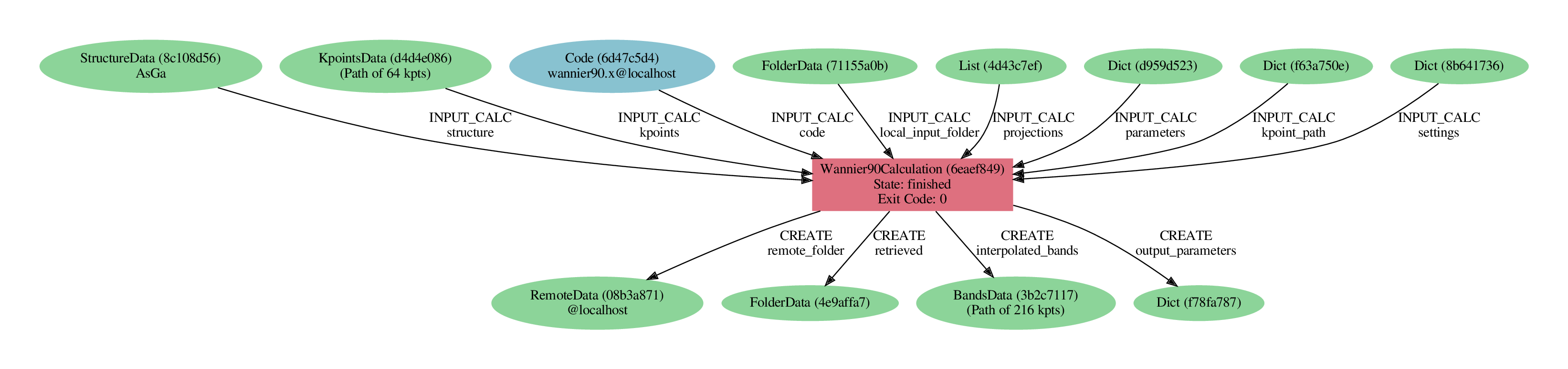
Fig. 2.11 Provenance graph for a single Wannier90 calculation.
You can generate such a provenance graph for any calculation or data in AiiDA by running:
verdi node graph generate <PK>
Try to reproduce the figure using the PK of your calculation (note that in our figure, we have used the
--ancestor-depth=1 option of verdi node graph generate to only show direct inputs; if you don’t, you will see
also the full provenance of the data, similar to the previous figure shown earlier).
You might wonder what happened under the hood, e.g. where to find the actual input and output files of the calculation. You will learn more about this in some of the advanced tutorials on AiiDA – for now, here are a few useful commands:
verdi calcjob inputcat <PK>  # shows the input file of the calculation
verdi calcjob outputcat <PK>  # shows the output file of the calculation
verdi calcjob res <PK>  # shows the parsed output
- Exercise: Here are a few questions you can now answer using these commands (try to check both the raw output and the parsed output)
What are the values of the various components of the spread \(\Omega_I\), \(\Omega_D\), \(\Omega_{OD}\)?
How many Wannier functions have been computed?
Was there any warning?
2.3.1. Understanding the launcher script
Above, we have just provided you a script that submits a calculation. Let us now check in detail some relevant sections, and how the input information got converted into the Wannier90 raw input file.
2.3.1.1. Choosing a structure
In this simple example, we load a structure already stored in the AiiDA database
(it is the one we imported from a file earlier on).
We do this using the load_node command (that accepts
either an integer PK or a string UUID).
2.3.1.2. Choosing the k-points
Also for kpoints, we are loading these from file. The reason is that we
already executed the Quantum ESPRESSO NSCF run, and we need to be sure that the order
of the k-points is the same (exercise: check in Fig. 2.10 that the
KpointsData node that we are using is indeed the input KpointsData
of the NSCF calculation). Otherwise, one can create an AiiDA KpointsData
and use the set_kpoints method to pass a \(N\times 3\) numpy array,
where \(N\) is the number of k-points.
2.3.1.3. Setting up input parameters
One very important input node is the parameters node, containing the input
flags for the code.
parameters = Dict(
   dict={
      'bands_plot': True,
      ...
   })
In particular, parameters is a Dict node, i.e.,
an AiiDA node containing a dictionary of key-value pairs (stored in the AiiDA
database and that can be easily queried - we will not see how to run queries in this
tutorial, but you can check the AiiDA documentation on querying or the full tutorial
for more information on this).
Exercise: Use verdi calcjob inputcat <PK> (using the PK of the calc job)
and check how the information in the parameters has been converted
into the Wannier90 input file.
2.3.1.4. Setting up the projections
In aiida-wannier90, there are two ways to set up projections.
Here, we are using the simplest approach (i.e., a list of strings, that are simply
inserted in the corresponding section of the raw input file). Similarly to a Dict node,
these strings are wrapped in a List AiiDA node, so that it gets stored and are queryable.
We will see a second (more easily queryable) way later on during this tutorial.
2.3.1.5. Setting up an (optional) list of k-points for the band plot
The path to compute an (interpolated) band structure needs to be specified
as a Dict node, contianing two keys: point_coords (a dictionary
with high-symmetry point labels and coordinates), and a path
(a list of pairs of labels, to indicate band-path segments):
kpoint_path = Dict(
   dict={
      'point_coords': {
            'GAMMA': [0.0, 0.0, 0.0],
            'L': [0.5, 0.5, 0.5],
            'X': [0.5, 0.0, 0.5]
      },
      'path': [('L', 'GAMMA'), ('GAMMA', 'X')]
   }
)
Exercise: Check how this has been converted into the raw input file.
2.3.1.6. Setting up the (optional) calculation settings
While often you don’t need to specify additional control parameters, there are cases in which you want to specify additional options to tune the way AiiDA will run the code.
You can find the full documentation of accepted keys for the settings
in the aiida-wannier90 documentation (e.g. to specify random projections,
or to retrieve/not retrieve specific files at the end of the run).
One important option that you will use very often is the flag postproc_setup:
if set to True, it will run a Wannier90 post-processing run (i.e., wannier90.x -pp).
In our case, do_preprocess is False so this is not set, but you would need
to run it in a full calculation including a DFT code.
# Settings node, with additional configuration
settings_dict = {}
if do_preprocess:
   settings_dict.update(
      {'postproc_setup': True}
   )
2.3.1.7. Setting up all inputs in a builder
Once you have created the nodes or loaded them from the database, you need to prepare a calculation, connect all inputs and then run (or submit it).
This is done creating a new calculation builder from a code: builder = code.get_builder().
Then, all inputs are attached to the builder as follows:
builder.structure = structure
builder.projections = projections
builder.parameters = parameters
...
Finally, you can:
runthe calculation (this stops the interpreter at that line, until the simulation is done, and then the execution of the python script continues):from aiida.engine import run results = run(builder)
At the end, you will get a dictionary of
results, one for every output node.If you want to run the calculation, but also get a reference to the
CalcJobNodethat represents the execution, you can use instead:from aiida.engine import run_get_node results, calcjobnode = run_get_node(builder)
If you want to submit to the daemon (what is done in the example above), you can use instead:
from aiida.engine import submit
calcjobnode = submit(builder)
In this case, you just get immediately a reference to the
CalcJobNode(not yet completed) and you can continue with the execution of the python script. This is useful e.g. if you want to submit many independent calculations at once in aforloop, and then let them run in parallel.
2.4. From calculations to workflows
AiiDA can help you run individual calculations but it is really designed to help you run workflows that involve several calculations, while automatically keeping track of the provenance for full reproducibility.
As the final step, we are going to launch the MinimalW90WorkChain workflow, a demo workflow
shipped with the aiida-wannier90 plugin, that also takes care of running the preliminary DFT
steps using Quantum ESPRESSO.
Here is a submission script that we are going to use:
from aiida.engine import run
from aiida.orm import Str, Dict, KpointsData, StructureData, load_code
from aiida.plugins import WorkflowFactory

from aiida_wannier90.orbitals import generate_projections


pw_code=load_code("<CODE LABEL>")  # Replace with the QE pw.x code label
wannier_code=load_code("<CODE LABEL>")  # Replace with the Wannier90 wannier.x code label
pw2wannier90_code=load_code("<CODE LABEL>")  # Replace with the QE pw2wannier90.x code label
pseudo_family_name="<UPF FAMILY NAME>" # Replace with the name of the pseudopotential family for SSSP efficiency


# GaAs structure
a = 5.68018817933178  # angstrom
structure = StructureData(
    cell=[[-a / 2., 0, a / 2.], [0, a / 2., a / 2.], [-a / 2., a / 2., 0]]
)
structure.append_atom(symbols=['Ga'], position=(0., 0., 0.))
structure.append_atom(symbols=['As'], position=(-a / 4., a / 4., a / 4.))

# 4x4x4 k-points mesh for the SCF
kpoints_scf = KpointsData()
kpoints_scf.set_kpoints_mesh([4, 4, 4])

# 10x10x10 k-points mesh for the NSCF/Wannier90 calculations
kpoints_nscf = KpointsData()
kpoints_nscf.set_kpoints_mesh([10, 10, 10])

# k-points path for the band structure
kpoint_path = Dict(dict={
    'point_coords': {
        'GAMMA': [0.0, 0.0, 0.0],
        'K': [0.375, 0.375, 0.75],
        'L': [0.5, 0.5, 0.5],
        'U': [0.625, 0.25, 0.625],
        'W': [0.5, 0.25, 0.75],
        'X': [0.5, 0.0, 0.5]
    },
    'path': [('GAMMA', 'X'), ('X', 'U'), ('K', 'GAMMA'),
             ('GAMMA', 'L'), ('L', 'W'), ('W', 'X')]
})

# sp^3 projections, centered on As
projections = generate_projections(
    [
        {
            'position_cart' :(-a / 4., a / 4., a / 4.),
            'ang_mtm_l_list': -3,
            'spin': None,
        },
    ],
    structure=structure
)

# Load the workflow
MinimalW90WorkChain = WorkflowFactory('wannier90.minimal')

# Run the workflow
run(
    MinimalW90WorkChain,
    pw_code=pw_code,
    wannier_code=wannier_code,
    pw2wannier90_code=pw2wannier90_code,
    pseudo_family=Str(pseudo_family_name),
    structure=structure,
    kpoints_scf=kpoints_scf,
    kpoints_nscf=kpoints_nscf,
    kpoint_path=kpoint_path,
    projections=projections
)
Download the demo_bands.py snippet.
You will need to edit the first lines, specifying the name of the AiiDA codes for Quantum ESPRESSO executables
pw.x and pw2wannier90.x, and for the Wannier90 code (that you can discover
as usual with verdi code list).
Moreover, you need to specify which pseudopotentials you want to use. AiiDA comes with tools to manage
pseudopotentials in UPF format (the format used by Quantum ESPRESSO and a few more codes), and to group them
in “pseudopotential families”. You can list all existing ones with verdi data upf listfamilies. We want
to use the SSSP library version 1.1.
Find the family you want to use and specify its name in the appropriate variable.
Exercise: Inspect the rest of the script to see how we are specifying inputs. In particular:
Note how you can define a crystal structure directly in AiiDA, without using any external library, if you know the cell vectors and the atoms coordinates.
Note how you can define a
KpointsDatanode (kpoints_scf) that does not include an explicit list of k-points, but rather represents a regular grid (\(4\times4\times4\) in this example, and similarly \(10\times10\times10\) forkpoints_nscf). The workflow, internally, knows that for the NSCF step one needs to unfold this k-points grid in an explicit grid of all k-points.Note a different way to specify the projections, using a more declarative format as a list of projection declarations (that gets internally converted in a queryable
OrbitalData, rather than just a list of strings). The documentation of theget_projectionsfunction and its parameters can be found here.
Once you have saved your changes, you can run the workflow with:
verdi run demo_minimal_w90_workchain.py
This workflow will:
Run a SCF simulation on GaAs
Run an NSCF calculation on a denser grid (with an explicit list of k-points)
Run a post-process Wannier90
-ppcalculation to get the.nnkpfileRun the interface code
pw2wannier90.xRun the Wannierisation step, returning the interpolated bands.
The workflow should take ~5 minutes on a typical laptop.
You may notice that verdi process list now shows more than one entry.
While you wait for the workflow to complete, let’s start exploring its provenance.
The full provenance graph obtained from verdi node graph generate will already be rather complex (you can try!),
so let’s try browsing the provenance interactively instead.
In a new verdi shell, start the AiiDA REST API:
verdi restapi
and open the Materials Cloud provenance browser (from the browser inside the virtual machine).
Note
The provenance browser is a Javascript application provided by Materials Cloud that connects to your AiiDA REST API. Your data never leave your computer.
Browse your AiiDA database.
Start by finding your workflow (in the left menu, filter the nodes by selecting
Process -> Workflow -> WorkChain. WorkChains are a specific type of workflows in AiiDA that allow to define multiple steps and can be paused and restarted between steps).Inspect the inputs and returned outputs of the workflow in the provenance browser (outputs will appear once the calculations are done). Moreover, you can inspect the calculations that the workflow launched, and check both their input and output nodes (via the provenance browser), as well as the raw inputs and outputs of the calculation (in the page of a specific
CalcJobNode).
Note
When perfoming calculations for a research project, at the end upon publication you can export your provenance graph using verdi export create and upload it to the Materials Cloud Archive, enabling your peers to explore the provenance of your calculations.
Once the workchain is finished, use verdi process show <PK> to inspect the MinimalW90WorkChain and find the PK of its interpolated_bands output.
Use this to produce an xmgrace output of the interpolated band structure:
verdi data bands export --format agr --output wannier_bands.agr <PK>
that you can then visualise using xmgrace wannier_bands.agr.
2.5. How to continue from here
The following appendix to this chapter discusses a bit more in detail how to import and export crystal structures from an AiiDA database, and which tools exist to obtain the primitive structure from a conventional structure, or more generally from a supercell.
Importantly, the conversion of a crystal structure (conventional cell)
to a primitive cell means the creation of a Data node from another Data node
using a python function. The appendix shows how easy it is with AiiDA to
wrap python functions into AiiDA’s calcfunctions that automatically
preserve the provenance of the data transformation in the AiiDA graph.
If you do not have time right now, you can jump directly to the next tutorial section, where we will see how to use fully automated AiiDA workflows that can obtain Wannier functions of a material with minimal input, without the need to specifying input parameters apart from the crystal structure and the code to run (and where even the choice of initial projections is automated).
2.6. Appendix: Get the primitive structure while preserving the provenance
Let us begin by downloading a gallium arsenide (GaAs) structure from the Crystallography Open Database and importing it into AiiDA.
Note
You can view the structure online.
wget http://crystallography.net/cod/9008845.cif
verdi data structure import ase 9008845.cif
As before, you will get the PK of the imported structure.
We note that a StructureData can also be exported to file to various formats.
As an example, let’s export the structure in XSF format and visualize it
with XCrySDen:
verdi data structure export --format=xsf <PK> > exported.xsf
xcrysden --xsf exported.xsf
You should see the GaAs supercell (8 atoms) that we downloaded from the COD database (in CIF format), imported into AiiDA and exported back into a different format (XSF).
In particular, the structure that we imported (and converted from CIF to an explicit list of atoms) used the conventional cell with 8 atoms, rather than the primitive one (with 2 atoms only).
2.6.1. Getting the primitive structure
We will now use seekpath (that internally uses spglib), to obtain the primitive cell from the conventional one. Actually, seekpath does more: it will also standardise the orientation of the structure, and suggest the path for a band-structure calculation.
We will not use seekpath directly, but a wrapper for AiiDA, that converts to and from AiiDA data types automatically (in particular, it reads directly AiiDA data nodes, and returns AiiDA nodes). The full documentation of these wrapper methods can be found on this page.
As a first thing, in the terminal, open an ipython shell with the AiiDA environment pre-loaded. This can be achieved by running:
verdi shell
Note
If you prefer working in jupyter, you can do so.
Open your browser (the one with jupyter that you opened in the setup chapter of this tutorial), then create a new Python 3 notebook (with the button “New” in the top right of the jupyter page, and then select “Python 3”).
Give the notebook a name: click on the word “Untitled” at the top, then type a file name (e.g. “create_supercell”) and confirm.
The only additional thing you need to do is to load the AiiDA environment.
In the first code cell, type %aiida and confirm with Shift+ENTER.
You should get a confirmation message “Loaded AiiDA DB environment”. You can then work as usual in jupyter, adding the code in the following cells.
Now, in this ipython shell (or in jupyter), you can import the wrapper function (that internally uses seekpath) as:
from aiida.tools import get_kpoints_path
We now want to use it. As you can see in the documentation, you need to pass
as a parameter a StructureData node (in our case, the node that you imported earlier from COD).
To load a node in the ipython shell, use the following command:
structure = load_node(<PK>)
where <PK> is the of the StructureData node you imported earlier.
At this point you are ready to get the primitive structure:
seekpath_data = get_kpoints_path(structure)
primitive = seekpath_data['primitive_structure']
Exercise: Check that the primitive object is an AiiDA StructureData node, and that it is still
not stored in the database (you can just print it). Moreover, check that you indeed obtained a
primitive structure by inspecting the unit cell using
print(primitive.cell), and the list and position of the atoms with print(primitive.sites).
2.6.2. Preserving the provenance
AiiDA is focused on making it easy to track the provenance of your calculation, i.e., the history of how it
has been generated, by which calculation, and with which inputs.
If you were just to store the primitive StructureData node, you would lose its provenance.
Instead, AiiDA provides simple tools to store it automatically in the form of a graph, where nodes are either
data nodes (as the one we have just seen), or calculations (i.e., “black boxes” that get data as input,
and create new data as output). Links between nodes represent the logical relationship between calculations and
their inputs and outputs.
While we refer to the full AiiDA documentation for more in-depth explanations, here we show the simplest way to run a python function while keeping the provenance at the same time.
This can be achieved by using a calcfunction: this is a wrapper around python functions
(technically, a python function decorator) that takes care of storing the execution of that function in the graph.
To use it, you need first to create a simple function that gets one or more AiiDA nodes, and returns one AiiDA node
(or a dictionary of AiiDA nodes). Moreover, you need to decorate it as a calcfunction, so that when it will be run,
it will be stored in the database.
Here is the complete code:
from aiida.engine import calcfunction

@calcfunction
def get_primitive(input_structure):
    from aiida.tools import get_kpoints_path
    seekpath_data = get_kpoints_path(input_structure)
    return {
        'primitive_structure': seekpath_data['primitive_structure'],
        'seekpath_parameters': seekpath_data['parameters']
    }
Once you have defined the function, run it on the structure node you loaded earlier:
results = get_primitive(structure)
primitive = results['primitive_structure']
The first thing you can notice (by printing primitive) is that now this node
has been automatically stored.
Additionally, you can check who created it simply as creator_function = primitive.creator.
You can for instance check the name of the function that was run, using creator_function.attributes['function_name']
(this returns get_primitive, the name of the function that we decorated as a calc_function).
Moreover, you can check the inputs of this function.
Exercise: Use creator_function.inputs.input_structure to get the input of the function called input_structure
(the name is taken from the parameter name in the definition of the get_primitive function) and check that it
is the exact same node that you started from.
Exercise: Go in a bash shell (e.g., open a new terminal – remember to also enter the virtual environment using workon aiida!). You can inspect graphically the full provenance of a given node using
verdi node graph generate <PK>
where we suggest here to use the PK of the creator_function. The code will generate a PDF that you can
open, and that should look like the following image:
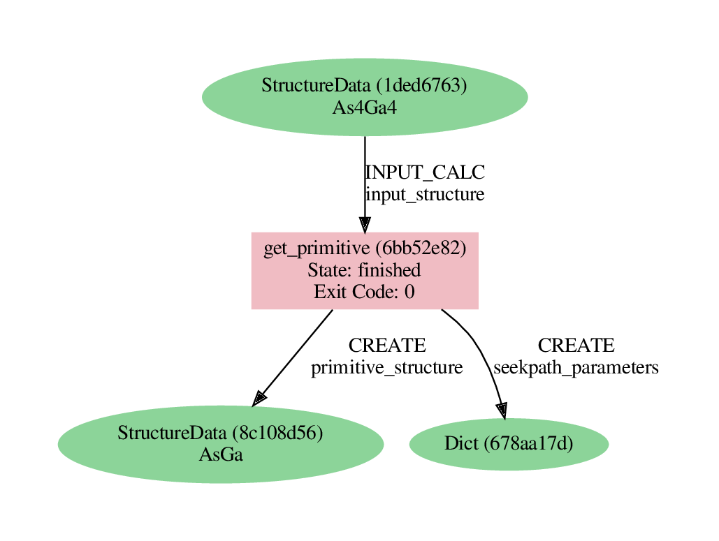
Fig. 2.12 Provenance graph for the calcfunction used to obtain the primitive structure of GaAs.
Note
TAKE HOME MESSAGE
AiiDA makes it very easy to convert python functions into calcfunctions that, every time
they are executed, represent their execution in the AiiDA graph.
The calc function itself is represented as a Calculation Node; all its function inputs and its (labeled) function outputs are also stored as AiiDA data nodes and are linked via INPUT and CREATE links, respectively.
It is possible to browse such graph, that tracks the provenance of the output data. Moreover, having the exact inputs tracked makes each calculation reproducible.
Finally (as we have already seen as an example in the previous sections for calculation jobs), outputs of a calculation can become inputs to a new calculation. Therefore, the AiiDA data provenance graph is a directed acyclic graph.
Note
While you can run the get_kpoints_path function as many times you want (and it will return
unstored nodes, so it will not clutter your AiiDA database), remember that every time you run the
get_primitive() calc function, you will get a bunch of new nodes in the database automatically stored for you.