2. A first taste of AiiDA

Let’s start with a quick demo of how AiiDA can make your life easier as a computational scientist.

We’ll be using the verdi command-line interface, which lets you manage your AiiDA installation, inspect the contents of your database, control running calculations and more.

As the first thing, open a terminal and type workon aiida to enter the “virtual environment” where AiiDA is installed. You will know that you are in the virtual environment because each new line will start with (aiida), e.g.:

(aiida) user@qe2019:~$

Note that you will need to retype workon aiida every time you open a new terminal.

Here are some first tasks for you:

• The verdi command supports tab-completion: In the terminal, type verdi, followed by a space and press the ‘Tab’ key twice to show a list of all the available sub commands.

• For help on verdi or any of its subcommands, simply append the --help/-h flag:

  verdi -h
  

2.1. Importing a structure and inspecting it

Let’s download a structure from the Crystallography Open Database and import it into AiiDA.

Note

You can view the structure online.

You can download the file and import it with the following two commands:

wget http://crystallography.net/cod/9008565.cif
verdi data structure import ase 9008565.cif

Each piece of data in AiiDA gets a PK number (a “primary key”) that identifies it in your database. This is printed out on the screen by the verdi data structure import command. Mark it down, as we are going to use it in the next commands.

Note

In the next commands, replace the string <PK> with the appropriate PK number.

Let us first inspect the node you just created:

verdi node show <PK>

You will get in output some information on the node, including its type (StructureData, the AiiDA data type for storing crystal structures), a label and a description (empty for now, can be changed), a creation time (ctime) and a last modification time (mtime), the PK of the node and its UUID (universally unique identifier).

Note

When should I use the PK and when should I use the UUID?

A PK is a short integer identifying the node and therefore easy to remember. However, the same PK number (e.g., PK=10) might appear in two different databases referring to two completely different pieces of data.

A UUID is a hexadecimal string that might look like this:

d11a4829-3e19-4978-bfcf-c28ddeb0891e

A UUID has instead the nice feature to be globally unique: even if you export your data and a colleague imports it, the UUIDs will remain the same (while the PKs will typically be different).

Therefore, use the UUID to keep a long-term reference to a node. Feel free to use the PK for quick, everyday use (e.g. to inspect a node).

Note

All AiiDA commands accepting a PK can also accept a UUID. Check this by trying the command before, this time with verdi node show <UUID>.

Note the following:

• AiiDA does not require the full UUID, but just the first part of it, as long as only one node starts with the string you provide. E.g., in the example above, you could also say verdi node show d11a4829-3e19. Most probably, instead, verdi node show d1 will return an error, since most probably you have more than one node starting with the string d1.

• By default, if what you pass is a valid integer, AiiDA will assume it is a PK; if at least one of the characters is not a digit, then AiiDA will assume it is (the first part of) a UUID.

• How to solve the issue, then, when the first part of the UUID is composed only by digits (e.g. in 2495301c-dd00-42d6-92e4-1a8c171bbb4a)? Indeed, using verdi node show 24953 would look for a node with PK=24953. As a solution, just add a dash, e.g. verdi node show 24953- so that AiiDA will consider this as the beginning of the UUID.

• Note that you can put the dash in any part of the string, and you don’t need to respect the typical UUID pattern with 8-4-4-4-12 characters per section: AiiDA will anyway first strip all dashes, and then put them back in the right place, so e.g. verdi node show 24-95-3 will give you the same result as verdi node show 24953-.

• Try to use again verdi node show on the StructureData node above, just with the first part of the UUID (that you got from the first call to verdi node show above).

• StructureData can be exported to file in various formats. As an example, let’s export the structure in XSF format and visualize it with XCrySDen:

  verdi data structure export --format=xsf <PK> > exported.xsf
  xcrysden --xsf exported.xsf
  

  You should be visualize to see the Si supercell (8 atoms) that we downloaded from the COD database (in CIF format), imported into AiiDA and exported back into a different format (XSF).

2.2. Running a calculation

The following short python script sets up a self-consistent field calculation for the Quantum ESPRESSO code:

"""Run SCF calculation with Quantum ESPRESSO"""
from aiida.orm.nodes.data.upf import get_pseudos_from_structure
from aiida.engine import submit

code = Code.get_from_string("<CODE LABEL>")  # REPLACE <CODE LABEL>
builder = code.get_builder()

# Select structure
structure = load_node(<STRUCTURE PK>)  # REPLACE <STRUCTURE PK>
builder.structure = structure

# Define calculation
parameters = {
  'CONTROL': {
    'calculation': 'scf',  # self-consistent field
  },
  'SYSTEM': {
    'ecutwfc': 30.,  # wave function cutoff in Ry
    'ecutrho': 240.,  # density cutoff in Ry
  },
}
builder.parameters = Dict(dict=parameters)

# Select pseudopotentials
builder.pseudos = get_pseudos_from_structure(structure, '<PP FAMILY>')  # REPLACE <PP FAMILY>

# Define K-point mesh in reciprocal space
KpointsData = DataFactory('array.kpoints')
kpoints = KpointsData()
kpoints.set_kpoints_mesh([4,4,4])
builder.kpoints = kpoints

# Set resources
builder.metadata.options.resources = {'num_machines': 1}

# Submit the job
calcjob = submit(builder)
print('Submitted CalcJob with PK=' + str(calcjob.pk))

Download the demo_calcjob.py script to your working directory. It contains a few placeholders for you to fill in:

1. the VM already has a number of codes preconfigured. Use verdi code list to find the label for the “PW” code and use it in the script.

2. replace the PK of the structure with the one you obtained

3. the VM already contains a number of pseudopotential families. Replace the PP family name with the one for the “SSSP efficiency” library found via verdi data upf listfamilies.

Then submit the calculation using:

verdi run demo_calcjob.py

From this point onwards, the AiiDA daemon will take care of your calculation: creating the necessary input files, running the calculation, and parsing its results.

In order to be able to do this, the AiiDA daemon must be running: to check this, you can run the command:

verdi daemon status

and, if the daemon is not running, you can start it with

verdi daemon start

It should take less than one minute to complete.

2.3. Analyzing the outputs of a calculation

Let’s have a look how your calculation is doing:

verdi process list  # shows only running processes
verdi process list --all  # shows all processes

Again, your calculation will get a PK, which you can use to get more information on it:

verdi process show <PK>

As you can see, AiiDA has tracked all the inputs provided to the calculation, allowing you (or anyone else) to reproduce it later on. AiiDA’s record of a calculation is best displayed in the form of a provenance graph

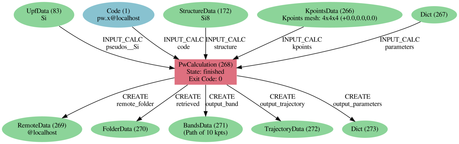
Fig. 2.19 Provenance graph for a single Quantum ESPRESSO calculation.

You can generate such a provenance graph for any calculation or data in AiiDA by running:

verdi node graph generate <PK>

Try to reproduce the figure using the PK of your calculation.

You might wonder what happened under the hood, e.g. where to find the actual input and output files of the calculation. You will learn more about this later – until then, here are a few useful commands:

verdi calcjob inputcat <PK>  # shows the input file of the calculation
verdi calcjob outputcat <PK>  # shows the output file of the calculation
verdi calcjob res <PK>  # shows the parsed output

A few questions you could answer using these commands (optional)

• How many atoms did the structure contain? How many electrons?

• How many k-points were specified? How many k-points were actually computed? Why?

• How many SCF iterations were needed for convergence?

• How long did Quantum ESPRESSO actually run (wall time)?

2.4. Moving to a different computer

Now, this Quantum ESPRESSO calculation ran on your (virtual) machine. This is fine for tests, but for production calculations you’ll typically want to run on a remote compute cluster. In AiiDA, moving a calculation from one computer to another means changing one line of code.

For the purposes of this tutorial, you’ll run on the machine at the IJS institute that you have already been using in the past days.

Note

In case you don’t have access to the IJS machine, you can instead use a cloud machine that we have setup on an OpenStack cluster in Switzerland (in the Swiss Supercomputing Centre CSCS), and that will be online (only) during the tutorial.

In this case, you will need to use the following files instead of the ones discussed below:

• Computer setup configuration file: openstack.yml

• Computer configure configuration file: openstack-config.yml

• Code setup configuration file: qe-openstack.yml

In order to know how to use them, continue reading through this section, replacing ijs with openstack. The code that you will create will be called qe-6.3-pw@openstack.

Download the ijs.yml setup template, that you can also see here:

---
label: ijs
description: Percolator machine at the Jožef Stefan Institute
hostname: percolator.ijs.si
transport: ssh  # connects via SSH
scheduler: slurm  # use SLURM scheduler
work_dir: "/home/{username}/aiida_run"
mpirun_command: "mpirun -np {tot_num_mpiprocs}"
mpiprocs_per_machine: "8"
shebang: "#!/bin/bash"
prepend_text: "#SBATCH --reservation=qe2019" # Needed to use the correct reservation in SLURM
append_text: " "

Read it to understand what is needed by AiiDA to setup a new computer. Then, let AiiDA know about this computer (that will be called ijs) by running:

verdi computer setup --config ijs.yml

Note

If you’re completing this tutorial at a later time and have no access to the percolator.ijs.si machine, simply use “localhost” instead as the hostname, and adapt the other parameters.

AiiDA is now aware of the existence of the computer but you’ll still need to let AiiDA know how to connect to it. AiiDA does this via SSH keys. Your tutorial VM already contains a private SSH key for connecting to the precolator.ijs.si machine that you set up on the first day of the tutorial, so all that is left is to configure it in AiiDA.

Download the ijs-config.yml configuration template, that looks like this:

---
username: <YOURUSERNAME> # <<< Replace with the username on percolator.ijs.si that you have setup on the first day of the tutorial
key_filename: "~/.ssh/id_rsa_nsc"
timeout: 30  # timout for SSH before giving up
key_policy: RejectPolicy  # Expect that you already connected once to the machine so it is in the known hosts, otherwise fail
safe_interval: 5  #  Minimum time (s) between consecutive connections

Replace the <YOURUSERNAME> placeholder with the username on percolator that you have been given the first day of the turorial, save the file and then run:

verdi computer configure ssh ijs --config ijs-config.yml --non-interactive

Note

Both verdi computer setup and verdi computer configure can be used interactively without configuration files, which are provided here just to avoid typing errors.

AiiDA should now have access to the percolator.ijs.si computer. Let’s quickly test this:

verdi computer test ijs

Finally, let AiiDA know about the code we are going to use. We’ve again prepared a template that looks as follows:

---
label: "qe-6.4.1-pw"
description: "quantum_espresso v6.4.1 (inside a Singularity container)"
input_plugin: "quantumespresso.pw"  # input plugin for pw.x code
computer: "ijs"
on_computer: true
remote_abs_path: "/opt/qe-6.4.1/pw.x"  # path to executable (inside singularity)
prepend_text: "ulimit -s unlimited"  # set stacksize to unlimited
append_text: " "

Download the qe.yml code template and run:

verdi code setup --config qe.yml
verdi code list  # note the label of the new code you just set up!

Now modify the code label in your demo_calcjob.py script to the label of your new code and simply run another calculation using verdi run demo_calcjob.py.

To see what is going on, AiiDA provides a command that lets you jump to the folder of the directory of the calculation on the remote computer:

verdi process list --all  # get PK of new calculation
verdi calcjob gotocomputer <PK>

Have a look around.

• Do you recognize the different files?

• Have a look at the submission script _aiidasubmit.sh. Compare it to the submission script of your previous calculation. What are the differences?

2.5. From calculations to workflows

AiiDA can help you run individual calculations but it is really designed to help you run workflows that involve several calculations, while automatically keeping track of the provenance for full reproducibility.

As the final step, we are going to launch the PwBandStructure workflow of the aiida-quantumespresso plugin.

"""Compute a band structure with Quantum ESPRESSO

Uses the PwBandStructureWorkChain provided by aiida-quantumespresso.
"""
from aiida.engine import submit
PwBandStructureWorkChain = WorkflowFactory('quantumespresso.pw.band_structure')

results = submit(
    PwBandStructureWorkChain,
    code=Code.get_from_string("<CODE LABEL>"), # REPLACE <CODE LABEL>
    structure=load_node(<PK>),  # REPLACE <PK>
)

Download the demo_bands.py snippet and run it using

verdi run demo_bands.py

This workflow will:

1. Determine the primitive cell of the input structure

2. Run a calculation on the primitive cell to relax both the cell and the atomic positions (vc-relax)

3. Refine the symmetry of the relaxed structure, and find a standardised primitive cell using SeeK-path

4. Run a self-consistent field calculation on the refined structure

5. Run a band structure calculation at fixed Kohn-Sham potential along a standard path between high-symmetry k-points determined by SeeK-path

The workflow uses the PBE exchange-correlation functional with suitable pseudopotentials and energy cutoffs from the SSSP library version 1.1.

The workflow should take ~10 minutes on your virtual machine. You may notice that verdi process list now shows more than one entry. While you wait for the workflow to complete, let’s start exploring its provenance.

The full provenance graph obtained from verdi node graph generate will already be rather complex (you can try!), so let’s try browsing the provenance interactively instead.

Start the AiiDA REST API:

verdi restapi

and open the Materials Cloud provenance browser (from the browser inside the virtual machine).

Note

As of September 2019, the Materials Cloud provenance browser is still being developed, so some features might still not be available or work as expected.

Note

The provenance browser is a Javascript application that connects to the AiiDA REST API. Your data never leaves your computer.

Browse your AiiDA database.

• Start by finding your Quantum ESPRESSO calculation (the type of node is called a CalcJobNode in AiiDA, since it is run as a job on a scheduler). Select Calculations in the left menu to filter for calculations only.

• Inspect the raw inputs and outputs of the calculation, and use the provenance browser to explore the input and output nodes of the calculation and the whole provenance of your simulations.

Note

When perfoming calculations for a publication, you can export your provenance graph using verdi export create and upload it to the Materials Cloud Archive, enabling your peers to explore the provenance of your calculations online.

Once the workchain is finished, use verdi process show <PK> to inspect the PwBandStructureWorkChain and find the PK of its band_structure output. Use this to produce a PDF of the band structure:

verdi data bands export --format mpl_pdf --output band_structure.pdf <PK>

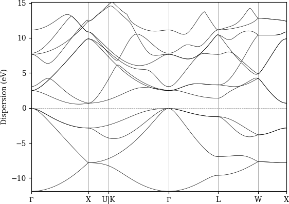
Fig. 2.20 Band structure computed by the PwBandStructure workchain.

Note

The BandsData node does contain information about the Fermi energy, so the energy zero in your plot will be arbitrary. You can produce a plot with the Fermi energy set to zero (as above) using the following code in a jupyter notebook:

%matplotlib inline
import aiida
aiida.load_profile()

from aiida.orm import load_node

scf_params = load_node(<PK>)  # REPLACE with PK of "scf_parameters" output
fermi_energy = scf_params.dict.fermi_energy

bands = load_node(<PK>)  # REPLACE with PK of "band_structure" output
bands.show_mpl(y_origin=fermi_energy, plot_zero_axis=True)

2.6. What next?

You now have a first taste of the type of problems AiiDA tries to solve. Here are some options for how to continue:

• Continue with the in-depth tutorial and learn more about the verdi, verdi shell and python interfaces to AiiDA. There is more than enough material to keep you busy for a day.

• Download Quantum Mobile virtual machine and try running the tutorial on your laptop instead. This will let you take the materials home and continue in your own time.

• Try setting up AiiDA directly on your laptop.

  Note

  For advanced Linux & python users only. AiiDA depends on a number of services and software that require some skill to set up. Unfortunately, we don’t have the human resources to help you solve issues related to your setup in a tutorial context.

• Continue your work from other parts of the workshop, chat with participants and enjoy yourself :-)