3. Automated high-throughput wannierisation
In the following tutorial you will learn how to perform automated high-throughput Wannierisation using a dedicated AiiDA workchain.
The protocol for automating the construction of Wannier functions is discussed in the following article:
Valerio Vitale, Giovanni Pizzi, Antimo Marrazzo, Jonathan Yates, Nicola Marzari, Arash Mostofi, Automated high-throughput wannierisation, accepted in npj Computational Materials (2020); https://arxiv.org/abs/1909.00433
whose data is available on the Materials Cloud Archive as:
Valerio Vitale, Giovanni Pizzi, Antimo Marrazzo, Jonathan R. Yates, Nicola Marzari, Arash A. Mostofi, Automated high-throughput Wannierisation, Materials Cloud Archive (2019), doi: 10.24435/materialscloud:2019.0044/v2.
The protocol leverages the SCDM method introduced in:
Anil Damle, Lin Lin, and Lexing Ying, Compressed representation of kohn–sham orbitals via selected columns of the density matrix Journal of Chemical Theory and Computation 11, 1463–1469 (2015).
Anil Damle and Lin Lin, Disentanglement via entanglement: A unified method for wannier localization, Multiscale Modeling & Simulation 16, 1392–1410 (2018).
The initial workflow was written by Antimo Marrazzo (EPFL) and Giovanni Pizzi (EPFL) (and is available, in a Virtual Machine, on the Materials Cloud entry mentioned above). It was later substantially improved and upgraded to AiiDA v1.x by Junfeng Qiao (EFPL). The SCDM implementation in Quantum ESPRESSO was done by Valerio Vitale (Imperial College London and University of Cambridge).
Note
Launch while you read! The workflow should take a few minutes to run on the virtual machine (5-10 minutes). So, we suggest that you launch it now (following the suggestions below) in the background, while you read through the tutorial.
3.1. Preparation
You can download the launch script for the workflow here: launch_auto-wannier_workflow.py.
The script accepts one argument, which is the location of the crystal structure file (in XSF format) for which you want to run the Wannierisation.
As an example, you can pick any one of the simple crystal structures from this list below:
Once you downloaded both the launcher script and one of the XSF files, first adapt the launcher script content, as usual, filling in the names of the codes that you want to use.
Then, launch the script with the following command:
verdi run launch_auto-wannier_workflow.py CsH.xsf
(in the following, we will use CsH as an example); you can replace CsH.xsf with any other structure of the list above, e.g. PtS2.xsf, or Br2Ti.xsf, …
3.2. Introduction
The use of maximally-localised Wannier functions (MLWFs) in high-throughput (HT) workflows has been hindered by the fact that generating MLWFs automatically and robustly without any user intervention and for arbitrary materials is, in general, very challenging.
The procedure to obtain MLWFs requires to specify a number of parameters that depends on the specific system under study, such as
the type of projections to build the \(A_{mn}({\mathbf{k}})\) matrix
and, in the case of entangled bands, many other parameters like
the number of Wannier functions,
the frozen energy window,
the outer energy window, …
The SCDM method allows to circumvent the need to specify initial projections, by introducting an algorithm that builds the \(A_{mn}({\mathbf{k}})\) matrix by optimally selecting columns of the density matrix \(P_{\mathbf{k}}\)
where \(f(\epsilon_{n\mathbf{k}})\) is an occupation function.
The SCDM algorithm is based on a QR factorization with column pivoting (QRCP) and it is
currently implemented in the pw2wannier90.x code of Quantum Espresso.
It is worth to stress that the occupation function does not necessarily correspond to a physical smearing, but it is used as a “window function” that restricts the manifold to the energy region of interest. For example, the isolated-band case can be recovered by setting \(f(\epsilon_{n\mathbf{k}})=1\) for energy values \(\epsilon_{n\mathbf{k}}\) within the energy range of the isolated bands, and zero elsewhere.
Another typical choice for the occupation function is the so-called complementary error function (erfc)
and it is used to to deal with a manifold of bands that are entangled only in the upper energy region (e.g. for metals, or for the conduction band of insulators). Another possible choice for the occupation function could be a Gaussian, for instance to extract bands in a specific energy range from a fully entangled manifold.
While the SCDM method allows to avoid the disentanglement procedure, and so the need to specify the frozen and outer window, it does not provide a recipe to set the smearing function parameters \(\mu\) and \(\sigma\). In addition, the number of Wannier functions remains to be set and a sensible value typically requires some chemical consideration, such as counting the number of atomic orbitals of a given orbital character (e.g. \(s\), \(p\), \(d\), \(sp^3\), …).
The Wannier90BandsWorkChain (distributed in the aiida-wannier90-workflows package) is an AiiDA workchain that implements a protocol that deals with the choice
of the number of Wannier functions and sets the parameters \(\mu\) and \(\sigma\) defining
the smearing function. For a full explanation of the protocol we refer to the article
Automated high-throughput wannierisation, while here we
just outline the main features.
The workflow starts by running a DFT calculation (with Quantum ESPRESSO) using automated workchains distributed within the aiida-quantumespresso plugin, that take care of automation for the calculations performed with Quantum ESPRESSO (QE). This is followed by a calculation of the projectability, that is the projection of the Kohn-Sham states onto localised atomic orbitals:
where the \(\phi_{Ilm}(\mathbf{k})\) are the pseudo-atomic orbitals (PAO) employed in the generation of the pseudopotentials, \(I\) is an index running over the atoms in the cell and \(lm\) define the usual angular momentum quantum numbers.
The workflow is designed for the specific use case where we are interested in wannierising the occupied bands (plus, optionally, some unoccupied or partially occupied bands) in insulators and in metals.
The number of Wannier functions is automatically set equal to the number of PAOs defined in the pseudopotentials (and the pseudopotentials are automatically taken from the SSSP efficiency library).
The projectabilities on these PAO orbitals are then computed and used to
set the optimal smearing function (erfc) parameters \(\mu\) and \(\sigma\), as explained in the paper
Automated high-throughput wannierisation.
After the calculation of the projectabilities, the workflow proceeds with the usual Wannierisation step: first
it computes the overlap and projection matrices using pw2wannier90, and then it runs the Wannier90 code.
Here we summarise the main steps of the Wannier90BandsWorkChain:
SCF (QuantumESPRESSO
pw.x)NSCF (QuantumESPRESSO
pw.x)Projectability (QuantumESPRESSO
projwfc.x)Wannier90 pre-processing (
wannier90.x -pp)Overlap matrices \(M_{mn}\), initial projections with SCDM \(A_{mn}\) (QuantumESPRESSO
pw2wannier90.x)Wannierisation (
wannier90.x)
The output of the workflow includes several nodes, among which the projectabilities and interpolated band structure, that we are going to inspect after the run.
3.3. Running the workflow
If you have not launch the script yet, please do it now!
Here we focus on how to run the Wannier90BandsWorkChain, the AiiDA workchain
that implements the automation workflow to obtain MLWFs.
Important note: For this tutorial, in order to keep the total simulation time down to ~5-10 minutes on a typical laptop, we run the workflow using the testing peotocol, where all the wavefunction cutoffs are halved to
speed up the calculations (with respect to the converged
and tested cutoffs suggested by the SSSP pseudopotential library). For production please use the theos-ht-1.0 protocol (or any other protocol with converged cutoffs).
We remind you that, to get a list of all the AiiDA processes (including calculations and workchains) that are running and their status you can use:
verdi process list
or alternatively
verdi process list -p1 -a
to see all workflows and calculations, even completed, that have been launched in the past 1 day.
Since you have already run the workflow by now, run the commands above to retrieve the corresponding PKs.
Here is the script that you have run:
#!/usr/bin/env runaiida
import sys
from aiida.orm import StructureData, Bool, Code, Dict
from aiida.engine import submit
from ase.io import read as aseread
from aiida_wannier90_workflows.workflows import Wannier90BandsWorkChain

# Codenames for pw.x, pw2wannier90.x, projwfc.x and wannier90.x
# Please modify these according to your machine
pw_code = Code.get_from_string("<CODE LABEL>")  # e.g. 'qe-6.5-pw@localhost'
pw2wan_code = Code.get_from_string("<CODE LABEL>")  # e.g. 'qe-6.5-pw2wannier90@localhost'
projwfc_code = Code.get_from_string("<CODE LABEL>")  # e.g. 'qe-6.5-projwfc@localhost'
wan_code = Code.get_from_string("<CODE LABEL>")  # e.g. 'wannier90-3.1.0-wannier@localhost'

# The 1st commandline argument specifies the structure to be calculated
xsf_file = sys.argv[1]  # e.g. 'CsH.xsf'

# Read xsf file and convert into a stored StructureData
structure = StructureData(ase=aseread(xsf_file))

# Prepare the builder to launch the workchain
builder = Wannier90BandsWorkChain.get_builder()
builder.structure = structure
builder.code = {
    'pw': pw_code,
    'pw2wannier90': pw2wan_code,
    'projwfc': projwfc_code,
    'wannier90': wan_code
}
# For this tutorial, we are using the 'testing' protocol,
# with all cutoffs halved, to speed up the simulations
builder.protocol = Dict(dict={'name': 'testing'})
# Flags to control the workchain behaviour
builder.controls = {
    # If True, compute only valence bands (NB: use for insulators only!)
    'only_valence': Bool(False),
    # If True, perform maximal-localisation (MLWF) procedure, i.e., minimise the spread Omega
    'do_mlwf': Bool(True),
}

# Submits the workchain
workchain = submit(builder)

print('launched WorkChain<{}> for structure {}'.format(workchain.pk, structure.get_formula()))
print("Use `verdi process list` or `verdi process show {}` to check the progress".format(workchain.pk))
Inspect the script in detail now, and make sure that you understand all its parts. The comments should guide you through it. As you will notice, the amount of information to provide to the workflow is really minimal: just the codes to use, the crystal structure, and some flags to control the behavior (which protocol to use, if you want to compute only valence bands, and if you want to run the MLWF step).
3.4. Analyzing the outputs of the workflow
Now we analyse the reports and outputs of the workflow using the command line.
Both while the Wannier90BandsWorkChain is running, and after its completion,
you can monitor its progress by
looking at its “report”, using the command
verdi process report <PK>
where <PK> corresponds to the workchain PK. You will see a list of log with messages produced by the workchain,
including the PKs of all its sub-workchains and of the calculations launched by the Wannier90BandsWorkChain.
The report will be similar to the following:
2020-03-19 07:58:27 [88  | REPORT]: [495|Wannier90BandsWorkChain|setup_protocol]: running the workchain with the "testing" protocol
2020-03-19 07:58:27 [89  | REPORT]: [495|Wannier90BandsWorkChain|setup]: workchain controls found in inputs: valence + conduction bands
2020-03-19 07:58:27 [90  | REPORT]: [495|Wannier90BandsWorkChain|run_seekpath]: running seekpath to get primitive structure for: CsH
2020-03-19 07:58:28 [91  | REPORT]: [495|Wannier90BandsWorkChain|setup_parameters]: number of machines 1 auto-set according to number of atoms
2020-03-19 07:58:30 [92  | REPORT]: [495|Wannier90BandsWorkChain|run_wannier_workchain]: launching Wannier90WorkChain<514>
2020-03-19 07:58:31 [93  | REPORT]:   [514|Wannier90WorkChain|run_scf]: scf step - launching PwBaseWorkChain<517> in scf mode
2020-03-19 07:58:33 [94  | REPORT]:     [517|PwBaseWorkChain|run_calculation]: launching PwCalculation<523> iteration #1
2020-03-19 07:58:46 [95  | REPORT]:     [517|PwBaseWorkChain|inspect_calculation]: PwCalculation<523> completed successfully
2020-03-19 07:58:46 [96  | REPORT]:     [517|PwBaseWorkChain|results]: work chain completed after 1 iterations
2020-03-19 07:58:46 [97  | REPORT]:     [517|PwBaseWorkChain|on_terminated]: remote folders will not be cleaned
2020-03-19 07:58:47 [98  | REPORT]:   [514|Wannier90WorkChain|inspect_scf]: scf PwBaseWorkChain successfully finished
2020-03-19 07:58:47 [99  | REPORT]:   [514|Wannier90WorkChain|run_nscf]: nscf number of bands set as 24
2020-03-19 07:58:48 [100 | REPORT]:   [514|Wannier90WorkChain|run_nscf]: nscf step - launching PwBaseWorkChain<537> in nscf mode
2020-03-19 07:58:49 [101 | REPORT]:     [537|PwBaseWorkChain|run_calculation]: launching PwCalculation<540> iteration #1
2020-03-19 08:01:16 [102 | REPORT]:     [537|PwBaseWorkChain|inspect_calculation]: PwCalculation<540> completed successfully
2020-03-19 08:01:16 [103 | REPORT]:     [537|PwBaseWorkChain|results]: work chain completed after 1 iterations
2020-03-19 08:01:16 [104 | REPORT]:     [537|PwBaseWorkChain|on_terminated]: remote folders will not be cleaned
2020-03-19 08:01:17 [105 | REPORT]:   [514|Wannier90WorkChain|inspect_nscf]: nscf PwBaseWorkChain successfully finished
2020-03-19 08:01:17 [106 | REPORT]:   [514|Wannier90WorkChain|should_do_projwfc]: SCDM mu & sigma are auto-set using projectability
2020-03-19 08:01:18 [107 | REPORT]:   [514|Wannier90WorkChain|run_projwfc]: projwfc step - launching ProjwfcCalculation<546>
2020-03-19 08:01:27 [108 | REPORT]:   [514|Wannier90WorkChain|inspect_projwfc]: projwfc ProjwfcCalculation successfully finished
2020-03-19 08:01:28 [109 | REPORT]:   [514|Wannier90WorkChain|run_wannier90_pp]: number of Wannier functions extracted from projections: 14
2020-03-19 08:01:29 [110 | REPORT]:   [514|Wannier90WorkChain|run_wannier90_pp]: wannier90 postproc step - launching Wannier90Calculation<559> in postproc mode
2020-03-19 08:01:35 [111 | REPORT]:   [514|Wannier90WorkChain|inspect_wannier90_pp]: wannier90 postproc Wannier90Calculation successfully finished
2020-03-19 08:01:38 [112 | REPORT]:   [514|Wannier90WorkChain|run_pw2wannier90]: pw2wannier90 step - launching Pw2Wannier90Calculation<567>
2020-03-19 08:02:16 [113 | REPORT]:   [514|Wannier90WorkChain|inspect_pw2wannier90]: Pw2wannier90Calculation successfully finished
2020-03-19 08:02:16 [114 | REPORT]:   [514|Wannier90WorkChain|run_wannier90]: wannier90 step - launching Wannier90Calculation<572>
2020-03-19 08:03:06 [115 | REPORT]:   [514|Wannier90WorkChain|inspect_wannier90]: Wannier90Calculation successfully finished
2020-03-19 08:03:06 [116 | REPORT]:   [514|Wannier90WorkChain|results]: final step - preparing outputs
2020-03-19 08:03:06 [117 | REPORT]:   [514|Wannier90WorkChain|results]: Wannier90WorkChain successfully completed
2020-03-19 08:03:07 [118 | REPORT]: [495|Wannier90BandsWorkChain|results]: wannier90 interpolated bands pk: 575
2020-03-19 08:03:07 [119 | REPORT]: [495|Wannier90BandsWorkChain|results]: Wannier90BandsWorkChain successfully completed
Once the workchain has finished to run, you can look at all its inputs and outputs with
verdi node show <PK>
You should obtain an output similar to what follows:
Property     Value
-----------  ------------------------------------
type         Wannier90BandsWorkChain
state        Finished [0]
pk           404
uuid         df46175b-4634-4edf-a303-e90af98a27fc
label
description
ctime        2020-03-18 18:38:36.294955+00:00
mtime        2020-03-18 18:50:59.245496+00:00
computer     [1] localhost

Inputs                          PK    Type
------------------------------  ----  -------------
code
    wannier90                   17    Code
    projwfc                     6     Code
    pw2wannier90                7     Code
    pw                          1     Code
controls
    kpoints_distance_for_bands  401   Float
    do_disentanglement          400   Bool
    plot_wannier_functions      399   Bool
    retrieve_hamiltonian        398   Bool
    auto_projections            397   Bool
    do_mlwf                     396   Bool
    only_valence                395   Bool
protocol                        403   Dict
structure                       402   StructureData

Outputs                         PK  Type
----------------------------  ----  --------------
nscf_parameters                454  Dict
primitive_structure            409  StructureData
projwfc_bands                  460  BandsData
projwfc_projections            459  ProjectionData
pw2wannier90_remote_folder     477  RemoteData
scf_parameters                 437  Dict
seekpath_parameters            407  Dict
wannier90_interpolated_bands   484  BandsData
wannier90_parameters           485  Dict
wannier90_remote_folder        482  RemoteData
wannier90_retrieved            483  FolderData

Called      PK  Type
--------  ----  ----------------
CALL       423  WorkChainNode
CALL       406  CalcFunctionNode

Log messages
---------------------------------------------
There are 7 log messages for this calculation
Run 'verdi process report 404' to see them
3.5. Analyzing and comparing the band structure
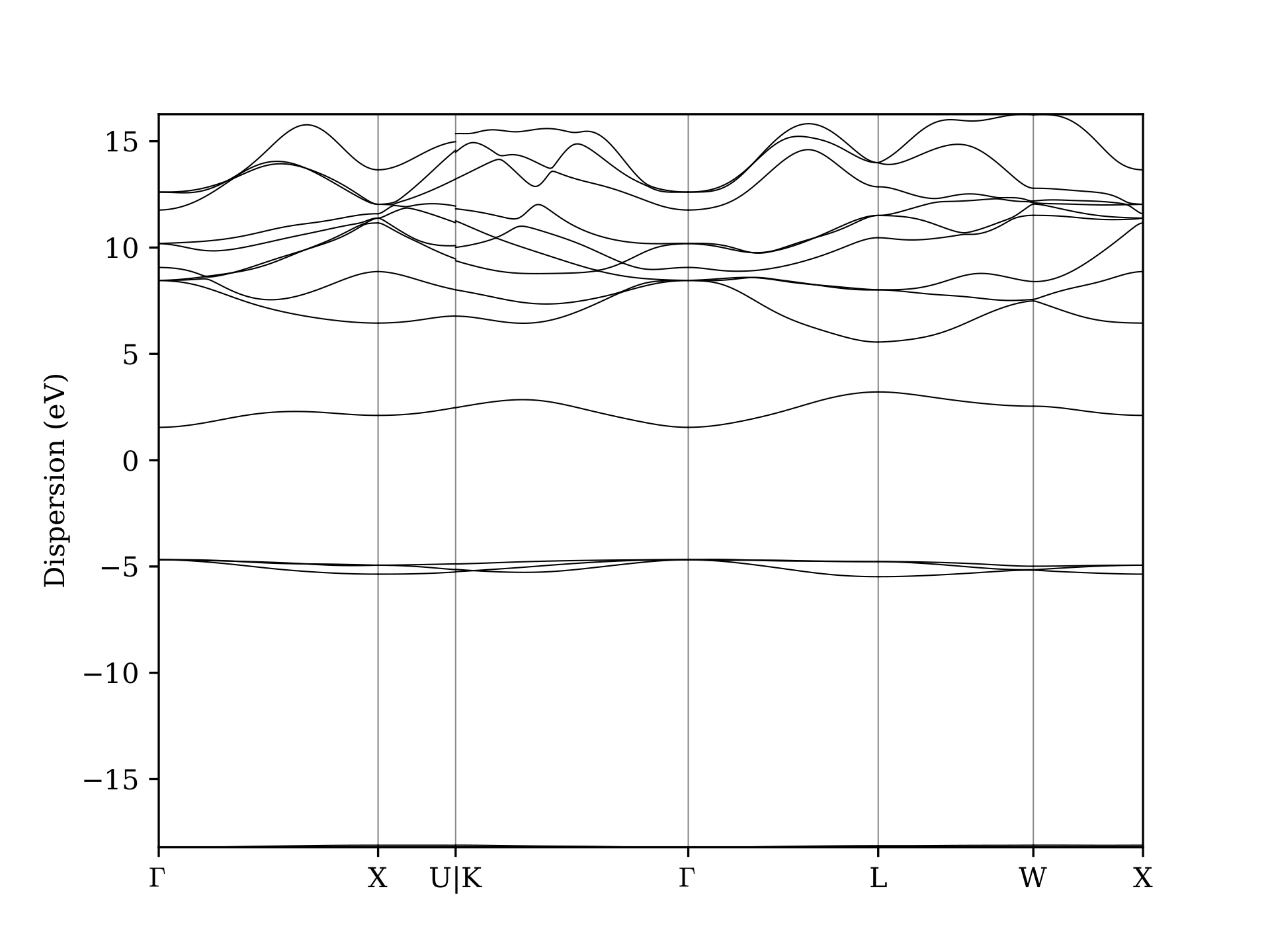
First let’s give a look at the interpolated band structure by exporting it to a PDF file with
verdi data bands export --format mpl_pdf --output band_structure.pdf <PK_bands>
where <PK_bands> stands for the BandsData PK produced by the workflow.
You can find it from the output of the verdi node show <PK> command
that you run before.
You should obtain a PDF like the following:
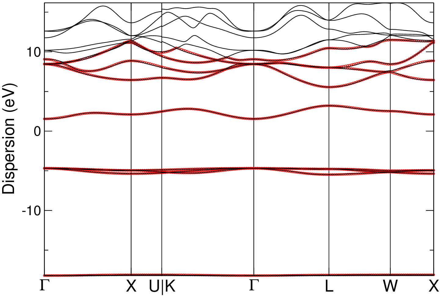
Now we compare the Wannier-interpolated bands with the full DFT bands calculation.
For convenience, we have already computed for you all the full DFT band structures for all the
compounds for which we provided the XSF above (even if you could easily recompute these band structures using
the plugins and workflows included in the aiida-quantumespresso package). You can download the full DFT bands in xmgrace format (.agr) form this list:
In particular, taking CsH as an example, you can first export the Wannier-interpolated bands that you just computed earlier in xmgrace format with
verdi data bands export --format agr --output CsH_wan_bands.agr <PK_bands>
and then you can compare them with the full DFT band structure using xmgrace typing:
xmgrace CsH_dft_bands.agr CsH_wan_bands.agr
where you can replace CsH with the correct chemical formula of the crystal structure that you used.
For reference, here are the two xmgrace files for CsH:
CsH_dft_bands.agr
CsH_wan_bands.agr.
In the case of CsH, you should obtain something like the following plot (note that we slightly updated the colors and graphical appearance of the plot with respect to the default one you would get by running the command above):
3.6. Analyzing the projectabilities
Now you will see how to look at the projectabilities that have been computed by the
workchain and then used to obtain \(\mu\) and \(\sigma\)
in the automation protocol.
You can download the following script
plot_projectabilities.py and run it
verdi run plot_projectabilities.py <PK>
where PK stands for the Wannier90BandsWorkChain pk.
You should obtain a plot similar to the following:
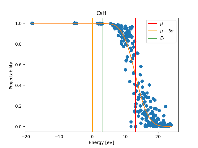
Exercise: Open the script and try to understand what it is doing.
As you can see, the protocol to choose \(\mu\) and \(\sigma\) ensures that the SCDM algorithm is applied to a density-matrix that includes (with a large weight) only those Kohn-Sham states that have a large projection on the manifold spanned by the PAOs.
3.7. Analyzing the provenance graph
We begin by generating the provenance graph with
verdi node graph generate <PK>
where the PK corresponds to the workflow you have just run. You should obtain something like the following:
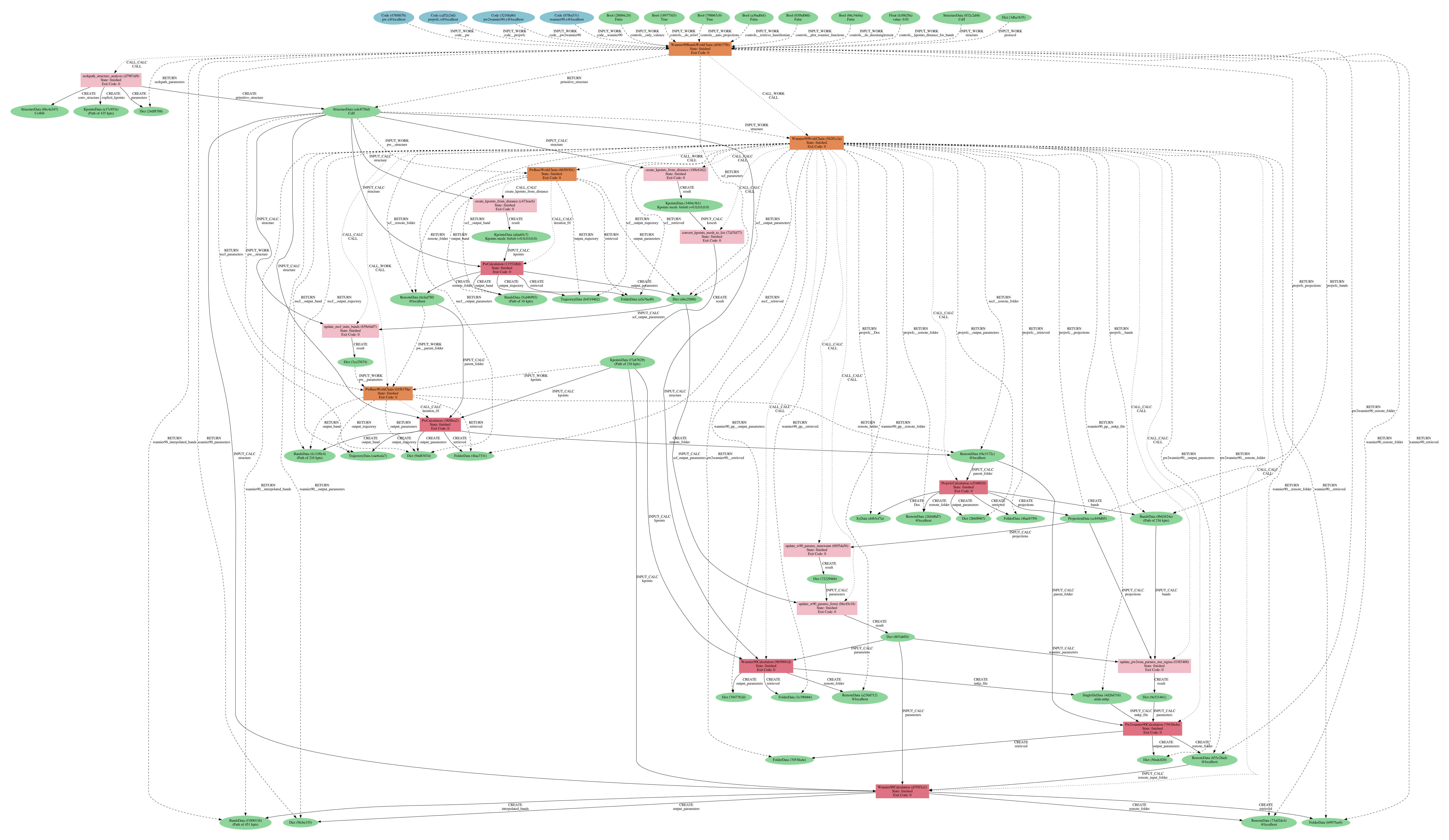
Fig. 3.2 Provenance graph for a single Wannier90BandsWorkChain run. (PDF version
CsH.dot.pdf)
As you can see, AiiDA has tracked all the inputs provided to all calculations (and their outputs), allowing you (or anyone else) to reproduce it later on.
3.8. (Optional) Maximal localisation and SCDM
Try to modify the launch_auto-wannier_workflow.py script to disable the MLWF
procedure in order to obtain Wannier functions with SCDM projections that are not maximally localised.
Exercise: Run the workflow for 1 or 2 materials of the dataset. Do you notice any difference when using or not the MLWF procedure? Which one gives better results? Do your results agree with the findings of the Automated high-throughput wannierisation paper?
3.9. (Optional) Browse your database with the REST API
Connect to the AiiDA REST API and browse your database! Follow the instructions that you find on the Materials Cloud website.
3.10. (Optional) More on AiiDA
You now have a first taste of the type of problems AiiDA tries to solve, and you have seen how it is possible, thanks to the tools provided by AiiDA, to develop plugins and workflows to automate your research tasks, while preserving the full provenance and guaranteeing reproducibility of your results.
Here are some options for how to continue:
Continue with the in-depth tutorial and learn more about the
verdi,verdi shellandpythoninterfaces to AiiDA. There is more than enough material to keep you busy for a day. You can check for instance the tutorial held in EPFL in May 2019 (note that this has been tested on a beta version of AiiDA 1.0 and we didn’t check yet if anything needs to be adapted for AiiDA 1.1, that you have in your VM).For advanced Linux & python users: try setting up AiiDA directly on your laptop. Note that AiiDA depends on a number of services and software that require some time to set up. Unfortunately, we will not have the time to help you solve issues related to your setup in a tutorial context, but you can refer to the AiiDA documentation and to the AiiDA mailing list.