1. Verdi command line
This part of the tutorial will familiarize you with the verdi command-line interface (CLI),
which lets you manage your AiiDA installation, inspect the contents of your database, control running calculations and more.
The
verdicommand supports tab-completion: In the terminal, typeverdi, followed by a space and press the ‘Tab’ key twice to show a list of all the available sub commands.For help on
verdior any of its subcommands, simply append the--help/-hflag, e.g.:verdi quicksetup -h
More details on verdi can be found in the online documentation.
1.1. Setting up a profile
After installing AiiDA, the first step is to create a “profile”. Typically, you would be using one profile per independent research project.
The easiest way of setting up a new profile is through verdi quicksetup.
Let’s set up a new profile that we will use throughout this tutorial:
verdi quicksetup
This will prompt you for some information, such as the name of the profile, your name, etc. The information about you as a user will be associated with all the data that you create in AiiDA and is important for attribution, when you start sharing your data with others. After you have answered all the questions, a new profile will be created, along with the required database and repository.
Note
verdi quicksetup is a user-friendly wrapper around the verdi setup command that provides more control over the profile setup.
As explained in the documentation, verdi setup expects certain external resources, such as the database to already have been pre-configured.
verdi quicksetup will try to do this for you, but may not be successful in certain environments.
To see this profile, and any others that may have been configured, run:
verdi profile list

Info: configuration folder: /home/max/.aiida
* generic
  quicksetup
Each line, generic and quicksetup in this example, corresponds to a profile.
The one marked with an asterisk is the “default” profile, meaning that any verdi command that you execute will be applied to that profile.
Note
The output you get may differ.
The generic profile is pre-configured on the virtual machine built for the tutorial (but we are not going to use it here).
Let’s change the default profile to the newly created quicksetup for the rest of the tutorial:
verdi profile setdefault quicksetup
From now on, all verdi commands will apply to the quicksetup profile.
Note
To quickly perform a single command on a profile that is not the default, use the -p/--profile option:
For example, verdi -p generic code list will display the codes for the generic profile, despite it not being the current default profile.
1.2. Importing data
Before we start running calculations ourselves, we are going to look at an AiiDA database already created by someone else. Let’s import one from the web:
verdi import https://object.cscs.ch/v1/AUTH_b1d80408b3d340db9f03d373bbde5c1e/marvel-vms/tutorials/aiida_tutorial_2019_05_perovskites_v0.3.aiida
Contrary to most databases, AiiDA databases contain not only results of calculations but also their inputs and information on how a particular result was obtained. This information, the data provenance, is stored in the form of a directed acyclic graph (DAG). In the following, we are going to introduce you to different ways of browsing this graph and will ask you to find out some information regarding the database you just imported.
1.3. Your first AiiDA graph
Fig. 1.13 shows a typcial example of a calculation represented in an AiiDA graph. Have a look to the figure and its caption before moving on.
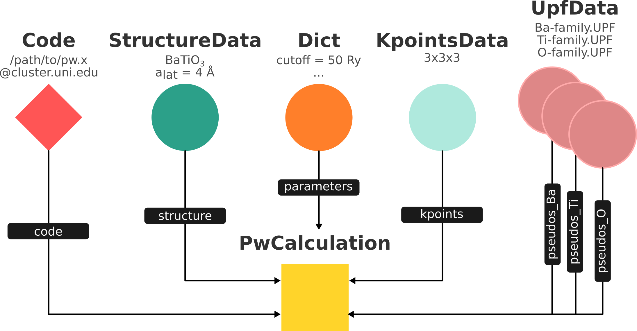
Fig. 1.13 Graph with all inputs (data, circles; and code, diamond) to the Quantum ESPRESSO calculation (square) that you will create in the Submit, monitor and debug calculations section of this tutorial.
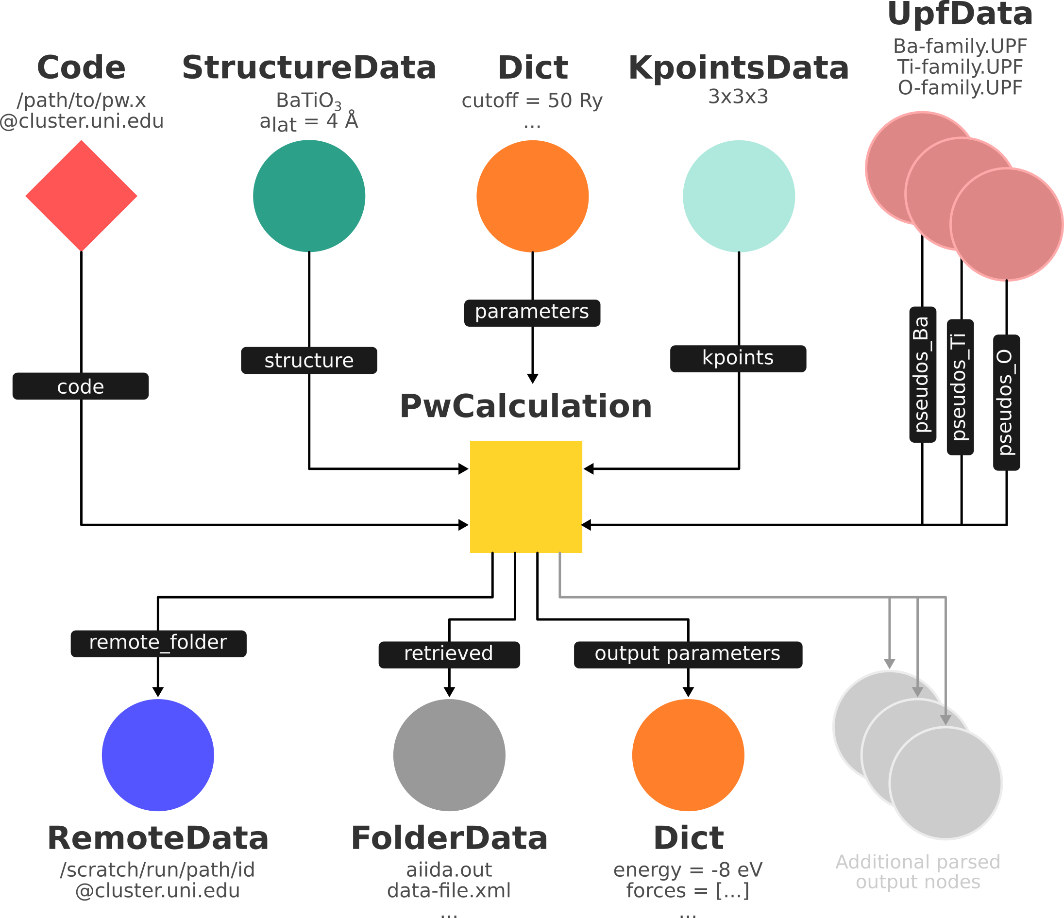
Fig. 1.14 Same as Fig. 1.13, but also with the outputs that the engine will create and connect automatically.
The RemoteData node is created during submission and can be thought as a symbolic link to the remote folder in which the calculation runs on the cluster.
The other nodes are created when the calculation has finished, after retrieval and parsing.
The node with linkname ‘retrieved’ contains the raw output files stored in the AiiDA repository; all other nodes are added by the parser.
Additional nodes (symbolized in gray) can be added by the parser (e.g. an output StructureData if you performed a relaxation calculation, a TrajectoryData for molecular dynamics etc.).
Fig. 1.13 was drawn by hand but you can generate a similar graph automatically by passing the identifier of a calculation node to verdi node graph generate <IDENTIFIER>.
Identifiers in AiiDA come in three forms:
“Primary Key” (PK): An integer, e.g.
723, that identifies your entity within your database (automatically assigned)Universally Unique Identifier (UUID): A string, e.g.
ce81c420-7751-48f6-af8e-eb7c6a30cec3that identifies your entity globally (automatically assigned)Label: A human-readable string, e.g.
test_qe_calculation(manually assigned)
Any verdi command that expects an identifier will accept a PK, a UUID or a label (although not all entities have a label by default).
While PKs are often shorter than UUIDs and can be easier to remember, they are only unique within your database.
Whenever you intend to share your data with others, use UUIDs to refer to nodes.
Note
For UUIDs, it is sufficient to specify a subset (starting at the beginning) as long as it can already be uniquely resolved.
For more information on identifiers in verdi and AiiDA in general, see the documentation.
For the remainder of this section, fields enclosed in angular brackets, such as <IDENTIFIER>, are placeholders that you should replace before executing the command.
With that in mind, let’s generate a graph for the calculation node with UUID ce81c420-7751-48f6-af8e-eb7c6a30cec3:
verdi node graph generate <IDENTIFIER>
This command will create the file <PK>.dot.pdf that can be viewed with any PDF document viewer.
You can open this file on the Amazon machine by using evince or, if the ssh connection is too slow, copy it via scp to your local machine.
To do so, if you are using Linux/Mac OS X, you can type in your local machine:
scp aiidatutorial:<path_with_the_graph_pdf> <local_folder>
and then open the file. Alternatively, you can use graphical software to achieve the same, for instance: WinSCP on Windows, Cyberduck on the Mac, or the ‘Connect to server’ option in the main menu after clicking on the desktop for Ubuntu.
1.4. The provenance browser
While the verdi CLI provides full access to the data underlying the provenance graph, a more intuitive tool for browsing AiiDA graphs is the interactive provenance browser available on Materials Cloud.
In order to use it, we first need to start the AiiDA REST API:
verdi restapi
 * Serving Flask app "aiida.restapi.run_api" (lazy loading)
 * Environment: production
   WARNING: Do not use the development server in a production environment.
   Use a production WSGI server instead.
 * Debug mode: off
 * Running on http://127.0.0.1:5000/ (Press CTRL+C to quit)
Now you can connect the provenance browser to your local REST API:
Open the provenance explorer on your laptop
In the form, paste the (local) URL
http://127.0.0.1:5000/api/v3of our REST APIClick “GO!”
Once the provenance browser javascript application has been loaded by your browser, it is communicating directly with the REST API and your data never leaves your computer.
Note
In order for this to work on your laptop, while the REST API is running on the virtual machine, we’ve enabled SSH tunneling for port 5000 in Connect to your virtual machine.
Start by clicking on the Details of a CalcJobNode and use the graph explorer to complete the exercise below.
If you ever get lost, just go to the “Details” tab, enter ce81c420-7751-48f6-af8e-eb7c6a30cec3 and click on the “GO” button.
Exercise
Use the provenance browser in order to figure out:
When was the calculation run and who run it?
Was it a serial or a parallel calculation? How many MPI processes were used?
What inputs did the calculation take?
What code was used and what was the name of the executable?
How many calculations were performed using this code?
1.5. Processes
Anything that ‘runs’ in AiiDA, be it calculations or workflows, is considered a Process.
To get a list of currently running processes, use:
verdi process list
Note
The first time you run this command, it might take a few seconds. Subsequent calls will be faster.
which should be empty:
PK    Created    Process label   Process State    Process status
----  ---------  --------------  ---------------  ----------------

Total results: 0

Info: last time an entry changed state: never
Let’s see whether there are any finished processes in the database by passing the -S/--process-state flag:
verdi process list -S finished
This command will list all the processes that have a process state Finished and should look something like:
PK    Created    Process label   Process State    Process status
----  ---------  --------------  ---------------  ----------------
1178  1653D ago  PwCalculaton    ⏹ Finished [0]
1953  1653D ago  PwCalculaton    ⏹ Finished [0]
1734  1653D ago  PwCalculaton    ⏹ Finished [0]
 336  1653D ago  PwCalculaton    ⏹ Finished [0]
1056  1653D ago  PwCalculaton    ⏹ Finished [0]
1369  1653D ago  PwCalculaton    ⏹ Finished [0]

Total results: 6

Info: last time an entry changed state: never
Processes can be in any of the following states:
Created
Waiting
Running
Finished
Excepted
Killed
The first three states are ‘active’ states, meaning the process is not done yet, and the last three are ‘terminal’ states. Once a process is in a terminal state, it will never become active again. The official documentation contains more details on process states.
In order to list processes of all states, use the -a/--all flag:
verdi process list -a
This command will list all the processes that have ever been launched.
As your database will grow, so will the output of this command.
To limit the number of results, you can use the -p/--past-days <NUM> option, that will only show processes that were created NUM days ago.
For example, this lists all processes launched since yesterday:
verdi process list -a -p1
Each row of the output identifies a process with some basic information about its status.
For a more detailed list of properties, you can use verdi process show, but to address any specific process, you need an identifier for it.
Let’s revisit the process with the UUID ce81c420-7751-48f6-af8e-eb7c6a30cec3, this time using the CLI:
verdi process show ce81c420-7751-48f6-af8e-eb7c6a30cec
Producing the output:
Property       Value
-------------  ------------------------------------
type           CalcJobNode
pk             828
uuid           ce81c420-7751-48f6-af8e-eb7c6a30cec3
label
description
ctime          2014-10-27 17:51:21.781045+00:00
mtime          2019-05-09 14:10:09.307986+00:00
process state  Finished
exit status    0
computer       [1] daint

Inputs      PK    Type
----------  ----  -------------
pseudos
    Ba      611   UpfData
    O       661   UpfData
    Ti      989   UpfData
code        825   Code
kpoints     811   KpointsData
parameters  829   Dict
settings    813   Dict
structure   27    StructureData

Outputs                    PK  Type
-----------------------  ----  -------------
output_kpoints           1894  KpointsData
output_parameters          62  Dict
output_structure           61  StructureData
output_trajectory_array    63  ArrayData
remote_folder             357  RemoteData
retrieved                  60  FolderData
You can use the PKs shown for the inputs and outputs to get more information about those nodes.
Warning
Since the inputs and outputs are Data nodes, not Process nodes, use verdi node show instead.
1.5.1. Dict and CalcJobNode
Let’s investigate some of the nodes appearing in the graph.
From the inputs of the process, let’s choose the node of type Dict with input link name parameters and type in the terminal:
verdi data dict show <IDENTIFIER>
where <IDENTIFIER> is the PK of the node.
A Dict contains a dictionary (i.e. key–value pairs), stored in the database in a format ready to be queried.
We will learn how to run queries later on in this tutorial.
The command above will print the content dictionary, containing the parameters used to define the input file for the calculation.
You can compare the dictionary with the content of the raw input file to Quantum ESPRESSO (that was generated by AiiDA) via the command:
verdi calcjob inputcat <IDENTIFIER>
where you provide the identifier of the calculation node.
Check the consistency of the parameters written in the input file and those stored in the Dict node.
Even if you don’t know the meaning of the input flags of a Quantum ESPRESSO calculation, you should be able to see how the input dictionary has been converted to Fortran namelists.
The previous command just printed the content of the ‘default’ input file aiida.in.
To see a list of all the files used to run a calculation (input file, submission script, etc.) instead type:
verdi calcjob inputls <IDENTIFIER>
Adding a --color flag allows you to easily distinguish files from folders by a different coloring.
Once you know the name of the file you want to visualize, you can call the verdi calcjob inputcat [PATH] command specifying the path.
For instance, to see the submission script, you can do:
verdi calcjob inputcat <IDENTIFIER> _aiidasubmit.sh
1.5.2. StructureData
Now let us focus on StructureData objects, which represent a crystal structure.
We can consider for instance the input structure to the calculation we were considering before (it should have the UUID 3a4b1270).
Such objects can be inspected interactively by means of an atomic viewer such as the one provided by ase.
AiiDA however supports several other viewers such as xcrysden, jmol, and vmd.
Type in the terminal:
verdi data structure show --format ase <IDENTIFIER>
to show the selected structure, although it will take a few seconds to appear You should be able to rotate the view with the right mouse button.
Note
If you receive some errors, make sure you started your SSH connection with the -X or -Y flag.
Alternatively, especially if showing them interactively is too slow over SSH, you can export the content of a structure node in various popular formats such as xyz or xsf.
This is achieved by typing in the terminal:
# verdi data structure export --format xsf <IDENTIFIER> > <IDENTIFIER>.xsf
verdi data structure export --format xsf 254e5a86 > 254e5a86.xsf
You can open the generated xsf file and observe the cell and the coordinates.
Then, you can then copy <IDENTIFIER>.xsf from the Amazon machine to your local one and then visualize it, e.g. with xcrysden (if you have it installed):
xcrysden --xsf <IDENTIFIER>.xsf
1.5.3. Codes and computers
Let us focus now on the nodes of type Code.
A code represents (in the database) the actual executable used to run the calculation.
Find the identifier of such a node in the graph and type:
verdi code show <IDENTIFIER>
The command prints information on the plugin used to interface the code to AiiDA, the remote machine on which the code is executed, the path of its executable, etc. To show a list of all available codes type:
verdi code list
If you want to show all codes, including hidden ones and those created by other users, use verdi code list -a -A.
Now, among the entries of the output you should also find the code just shown.
Similarly, the list of computers on which AiiDA can submit calculations is accessible by means of the command:
verdi computer list -a
The -a flag shows all computers, also the one imported in your database but that you did not configure, i.e. to which you don’t have access.
Details about each computer can be obtained by the command:
verdi computer show <COMPUTERNAME>
Now you have the tools to answer the question: what is the scheduler installed on the computer where the calculations of the graph have run?
1.5.4. Calculation results
The results of a calculation can be accessed directly from the calculation node. Type in the terminal:
verdi calcjob res <IDENTIFIER>
which will print the output dictionary of the ‘scalar’ results parsed by AiiDA at the end of the calculation. Note that this is actually a shortcut for:
verdi data dict show <IDENTIFIER>
where IDENTIFIER refers to the Dict node attached as an output of the calculation node, with link name output_parameters.
By looking at the output of the command, what is the Fermi energy of the calculation with UUID ce81c420?
Similarly to what you did for the calculation inputs, you can access the output files via the commands:
verdi calcjob outputls <IDENTIFIER>
and
verdi calcjob outputcat <IDENTIFIER>
Use the latter to verify that the Fermi energy that you have found in the last step has been extracted correctly from the output file
Note
Hint: filter the lines containing the string ‘Fermi’, e.g. using grep, to isolate the relevant lines
The results of calculations are stored in two ways: Dict objects are stored in the database, which makes querying them very convenient, whereas ArrayData objects are stored on the disk.
Once more, use the command verdi data array show <IDENTIFIER> to determine the Fermi energy obtained from calculation with the UUID ce81c420.
This time you will need to use the identifier of the output ArrayData of the calculation, with link name output_trajectory_array.
As you might have realized the difference now is that the whole series of values of the Fermi energy calculated after each relax/vc-relax step are stored.
The choice of what to store in Dict and ArrayData nodes is made by the parser of pw.x implemented in the aiida-quantumespresso plugin.
1.5.5. (Optional section) Comments
AiiDA offers the possibility to attach comments to a any node, in order to be able to remember more easily its details.
Node with UUID prefix ce81c420 should have no comments, but you can add a very instructive one by typing in the terminal:
verdi node comment add "vc-relax of a BaTiO3 done with QE pw.x" -N <IDENTIFIER>
Now, if you ask for a list of all comments associated to that calculation by typing:
verdi node comment show <IDENTIFIER>
the comment that you just added will appear together with some useful information such as its creator and creation date.
We let you play with the other options of verdi node comment command to learn how to update or remove comments.
1.6. AiiDA groups of calculations
In AiiDA, calculations (and more generally nodes) can be organized in groups, which are particularly useful to assign a set of calculations or data to a common project. This allows you to have quick access to a whole set of calculations with no need for tedious browsing of the database or writing complex scripts for retrieving the desired nodes. Type in the terminal:
verdi group list -a -A
to show a list of all groups that exist in the database.
Choose the PK of the group named tutorial_pbesol and look at the calculations that it contains by typing:
verdi group show <IDENTIFIER>
In this case, we have used the name of the group to organize calculations according to the pseudopotential that has been used to perform them. Among the rows printed by the last command you will be able to find the calculation we have been inspecting until now.
If, instead, you want to know all the groups to which a specific node belongs, you can run:
verdi group list -N/--node <IDENTIFIER>