2. A first taste

Let’s start with a quick demo of how AiiDA can make your life easier as a computational scientist.

To get started, type workon aiida in your terminal to enter the virtual environment where AiiDA is installed. You have entered the the virtual environment when the prompt starts with (aiida), e.g.:

(aiida) username@hostname:~$

Note

You need to retype workon aiida whenever you open a new terminal.

We’ll be using the verdi command-line interface, which lets you manage your AiiDA installation, inspect the contents of your database, control running calculations and more.

Here are some first tasks for you:

• The verdi command supports tab-completion: In the terminal, type verdi, followed by a space and press the ‘Tab’ key twice to show a list of all the available sub commands.

• For help on any verdi command, simply append the --help/-h flag:

  verdi -h
  

2.1. Getting help

There are a number of helpful resources available to you for getting more information about AiiDA. Please consider:

• consulting the extensive AiiDA documentation

• asking in the Slack channel of the tutorial

• asking your neighbor

• asking a tutor

• opening a new issue on the tutorial issue tracker

2.2. Importing a structure and running a calculation

Let’s download a structure from the Crystallography Open Database and import it into AiiDA:

wget http://crystallography.net/cod/9008565.cif
verdi data structure import ase 9008565.cif

Each piece of data in AiiDA gets a PK number (a “primary key”) that identifies it in your database. The PK is printed to screen by the verdi data structure import command. Mark down the PK for your structure and use it to replace the <PK> placeholders in what follows.

Note

You can view the structure either online or use jmol 9008565.cif locally.

The following short python script sets up a self-consistent field calculation for the Quantum ESPRESSO code:

"""Run SCF calculation with Quantum ESPRESSO"""
from aiida.orm.nodes.data.upf import get_pseudos_from_structure
from aiida.engine import submit

code = Code.get_from_string("<CODE LABEL>")  # REPLACE <CODE LABEL>
builder = code.get_builder()

# Select structure
structure = load_node(<STRUCTURE PK>)  # REPLACE <STRUCTURE PK>
builder.structure = structure

# Define calculation
parameters = {
  'CONTROL': {
    'calculation': 'scf',  # self-consistent field
  },
  'SYSTEM': {
    'ecutwfc': 30.,  # wave function cutoff in Ry
    'ecutrho': 240.,  # density cutoff in Ry
  },
}
builder.parameters = Dict(dict=parameters)

# Select pseudopotentials
builder.pseudos = get_pseudos_from_structure(structure, '<PP FAMILY>')  # REPLACE <PP FAMILY>

# Define K-point mesh in reciprocal space
KpointsData = DataFactory('array.kpoints')
kpoints = KpointsData()
kpoints.set_kpoints_mesh([4,4,4])
builder.kpoints = kpoints

# Set resources
builder.metadata.options.resources = {'num_machines': 1}

# Submit the job
calcjob = submit(builder)
print('Submitted CalcJob with PK=' + str(calcjob.pk))

Download the demo_calcjob.py script to your working directory. It contains a few placeholders for you to fill in:

1. the VM already has a number of codes preconfigured. Use verdi code list to find the label for the “PW” code and use it in the script.

2. replace the PK of the structure with the one you obtained

3. the VM already contains a number of pseudopotential families. Replace the PP family name with the one for the “SSSP efficiency” library found via verdi data upf listfamilies.

Then submit the calculation using:

verdi run demo_calcjob.py

From this point onwards, the AiiDA daemon will take care of your calculation: creating the necessary input files, running the calculation, and parsing its results. It should take less than one minute to complete.

2.3. Analyzing the outputs of a calculation

Let’s have a look how your calculation is doing:

verdi process list  # shows only running processes
verdi process list --all  # shows all processes

Again, your calculation will get a PK, which you can use to get more information on it:

verdi process show <PK>

As you can see, AiiDA has tracked all the inputs provided to the calculation, allowing you (or anyone else) to reproduce it later on. AiiDA’s record of a calculation is best displayed in the form of a provenance graph

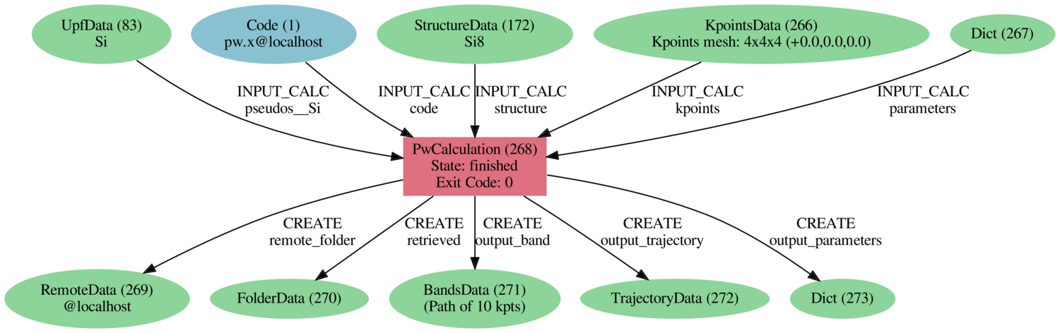
Fig. 2.17 Provenance graph for a single Quantum ESPRESSO calculation.

You can generate such a provenance graph for any calculation or data in AiiDA by running:

verdi node graph generate <PK>

Try to reproduce the figure using the PK of your calculation.

Note

By default, AiiDA uses UUIDs to label nodes in provenance graphs (more about UUIDs vs PKs later). Try using the -h option to figure out how to switch to the PK identifier.

You might wonder what happened under the hood, e.g. where to find the actual input and output files of the calculation. You will learn more about this later – until then, here are a few useful commands to try:

verdi calcjob inputcat <PK>  # shows the input file of the calculation
verdi calcjob outputcat <PK>  # shows the output file of the calculation
verdi calcjob res <PK>  # shows the parsed output

A few questions you could answer using these commands (optional)

• How many atoms did the structure contain? How many electrons?

• How many k-points were specified? How many k-points were actually computed? Why?

• How many SCF iterations were needed for convergence?

• How long did Quantum ESPRESSO actually run (wall time)?

2.4. Moving to a different computer

Now, this Quantum ESPRESSO calculation ran on your (virtual) machine. This is fine for tests, but for production calculations you’ll typically want to run on a remote compute cluster. In AiiDA, moving a calculation from one computer to another means changing one line of code.

For the purposes of this tutorial, you’ll run on your neighbor’s computer. Ask your neighbor for the IP address of their VM. Then, download the neighbor.yml setup template, replace the placeholder by the IP address and let AiiDA know about this computer by running:

verdi computer setup --config neighbor.yml

Note

If you’re completing this tutorial at a later time and have no partner machine, simply use “localhost” instead of the IP address.

AiiDA is now aware of the existence of the computer but you’ll still need to let AiiDA know how to connect to it. AiiDA does this via SSH keys. Your tutorial VM already contains a private SSH key for connecting to the compute user of your neighbor’s machine, so all that is left is to configure it in AiiDA.

Download the neighbor-config.yml configuration template and run:

verdi computer configure ssh neighbor --config neighbor-config.yml --non-interactive

Note

Both verdi computer setup and verdi computer configure can be used interactively without configuration files, which are provided here just to avoid typing errors.

AiiDA should now have access to your neighbor’s computer. Let’s quickly test this:

verdi computer test neighbor

Finally, let AiiDA know about the code we are going to use. We’ve again prepared a template that looks as follows:

---
label: "qe-6.4.1-pw"
description: "quantum_espresso v6.4.1"
input_plugin: "quantumespresso.pw"  # input plugin for pw.x code
computer: "neighbor"
on_computer: true
remote_abs_path: "/usr/local/bin/pw.x"  # path to executable
prepend_text: "ulimit -s unlimited"  # set stacksize to unlimited
append_text: " "

Download the qe.yml code template and run:

verdi code setup --config qe.yml
verdi code list  # note the label of the new code you just set up!

Now modify the code label in your demo_calcjob.py script to the label of your new code and simply run another calculation using verdi run demo_calcjob.py.

To see what is going on, AiiDA provides a command that lets you jump to the folder of the directory of the calculation on the remote computer:

verdi process list --all  # get PK of new calculation
verdi calcjob gotocomputer <PK>

Have a look around.

• Do you recognize the different files?

• Have a look at the submission script _aiidasubmit.sh. Compare it to the submission script of your previous calculation. What are the differences?

2.5. From calculations to workflows

AiiDA can help you run individual calculations but it is really designed to help you run workflows that involve several calculations, while automatically keeping track of the provenance for full reproducibility. As the final step, you are going to run such a workflow.

Let’s have a look at the workflows that are currently installed:

verdi plugin list aiida.workflows

The quantumespresso.pw.band_structure workflow from the aiida-quantumespresso plugin computes the electronic band structure for a given atomic structure. Let AiiDA tell you which inputs it takes and which outputs it produces:

verdi plugin list aiida.workflows quantumespresso.pw.band_structure

We have prepared a short python snippet that shows how to run this workflow.

"""Compute a band structure with Quantum ESPRESSO

Uses the PwBandStructureWorkChain provided by aiida-quantumespresso.
"""
from aiida.engine import submit
PwBandStructureWorkChain = WorkflowFactory('quantumespresso.pw.band_structure')

results = submit(
    PwBandStructureWorkChain,
    code=Code.get_from_string("qe-6.4.1-pw@localhost"),
    structure=load_node(<PK>),  # REPLACE <PK>
)

Download the demo_bands.py snippet, replace the PK, and run it using

verdi run demo_bands.py

This workflow will:

1. Determine the primitive cell of the input structure

2. Run a calculation on the primitive cell to relax both the cell and the atomic positions (vc-relax)

3. Refine the symmetry of the relaxed structure, and find a standardised primitive cell using SeeK-path

4. Run a self-consistent field calculation on the refined structure

5. Run a band structure calculation at fixed Kohn-Sham potential along a standard path between high-symmetry k-points determined by SeeK-path

The workflow uses the PBE exchange-correlation functional with suitable pseudopotentials and energy cutoffs from the SSSP library version 1.1.

The workflow should take ~10 minutes on your virtual machine. You may notice that verdi process list now shows more than one entry. While you wait for the workflow to complete, let’s start exploring its provenance.

The full provenance graph obtained from verdi node graph generate will already be rather complex (you can try!), so let’s try browsing the provenance interactively instead.

Start the AiiDA REST API:

verdi restapi

and open the Materials Cloud provenance browser.

Note

In order for the provenance browser to work, you need to configure SSH to tunnel port 5000 from your VM to your local laptop (see here Connect to your virtual machine).

The provenance browser is a Javascript application that connects to the AiiDA REST API. Your data never leaves your computer.

Browse your AiiDA database.

• Start by finding your structure in Data => Structure

• Use the provenance browser to explore the steps of the PwBandStructureWorkChain

Note

When perfoming calculations for a publication, you can export your provenance graph using verdi export create and upload it to the Materials Cloud Archive, enabling your peers to explore the provenance of your calculations online.

Once the workchain is finished, use verdi process show <PK> to inspect the PwBandStructureWorkChain and find the PK of its band_structure output. Use this to produce a PDF of the band structure:

verdi data bands export --format mpl_pdf --output band_structure.pdf <PK>

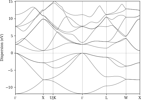
Fig. 2.18 Band structure computed by the PwBandStructure workchain.

Note

The BandsData node does contain information about the Fermi energy, so the energy zero in your plot will be arbitrary. You can produce a plot with the Fermi energy set to zero (as above) using the following code in a jupyter notebook:

%aiida
%matplotlib inline

scf_params = load_node(<PK>)  # REPLACE with PK of "scf_parameters" output
fermi_energy = scf_params.dict.fermi_energy

bands = load_node(<PK>)  # REPLACE with PK of "band_structure" output
bands.show_mpl(y_origin=fermi_energy, plot_zero_axis=True)

2.6. What next?

You now have a first taste of the type of problems AiiDA tries to solve.

Continue with the in-depth tutorial to learn more about the verdi, verdi shell and python interfaces to AiiDA.