1. Quantum ESPRESSO¶

Let’s start with a quick demo of how AiiDA can make your life easier as a computational scientist.

Note

Throughout this tutorial we will be using the verdi command line interface. Here’s couple of tricks that will make your life easier:

The verdi command supports tab-completion: In the terminal, type verdi, followed by a space and press the ‘Tab’ key twice to show a list of all the available sub commands.
For help on verdi or any of its subcommands, simply append the --help/-h flag:
```
$ verdi -h
```

1.1. Importing a structure and inspecting it¶

First, download the Si structure file: Si.cif. You can download the file to the AiiDAlab cluster using wget:

$ wget https://aiida-tutorials.readthedocs.io/en/tutorial-2020-bigmap-lab/_downloads/a40ce5fed92027564ab551dcc3e51774/Si.cif

Next, you can import it with the verdi CLI.

$ verdi data structure import ase Si.cif
  Successfully imported structure Si2 (PK = 171)

Each piece of data in AiiDA gets a PK number (a “primary key”) that identifies it in your database. This is printed out on the screen by the verdi data structure import command. It’s a good idea to mark it down, but should you forget, you can always have a look at the structures in the database using:

$ verdi data structure list
  Id  Label    Formula
----  -------  ---------
 105           Si2
 111           Si2
 112           Si8
 171           Si2

Total results: 4

The first column (marked Id) are the PK’s of the StructureData nodes.

Important

It is likely that the PK numbers shown throughout this tutorial are different for your database! Throughout this section, replace the string <PK> with the appropriate PK number.

Let us first inspect the node you just created:

$ verdi node show <PK>
Property     Value
-----------  ------------------------------------
type         StructureData
pk           171
uuid         ac3626d2-60ec-4e54-953f-7b7cf3716b16
label
description
ctime        2020-11-29 16:11:39.900886+00:00
mtime        2020-11-29 16:11:40.025347+00:00

You can see some information on the node, including its type (StructureData, the AiiDA data type for storing crystal structures), a label and a description (empty for now, can be changed), a creation time (ctime) and a last modification time (mtime), the PK of the node and its UUID (universally unique identifier). The PK and UUID both reference the node with the only difference that the PK is unique for your local database only, whereas the UUID is a globally unique identifier and can therefore be used between different databases.

Important

The UUIDs are generated randomly and are therefore guaranteed to be different from the ones shown here. In the commands that follow, replace <PK>, or <UUID> by the appropriate identifier.

1.2. Running a calculation¶

We’ll start with running a simple SCF calculation with Quantum ESPRESSO for the structure we just imported. Let’s first look at the codes in our database with the verdi shell:

$ verdi code list
# List of configured codes:
# (use 'verdi code show CODEID' to see the details)
* pk 1 - pw@localhost

We can see the code you set up during the AiiDAlab demo, with label pw, set up on the localhost computer.

To run the SCF calculation, we’ll also need to provide the family of pseudopotentials. To see the list of installed pseudopotential families, do:

$ verdi data upf listfamilies
Success: * SSSP_1.1_efficiency [85 pseudos]
Success: * SSSP_1.1_precision [85 pseudos]

Along with the PK of the StructureData node for the silicon structure we imported in the previous section, we now have everything to set up the calculation step by step. We will do this in the verdi shell, an interactive IPython shell that has many basic AiiDA classes pre-loaded. To start the IPython shell, simply type in the terminal:

$ verdi shell

First, we’ll load the code from the database using its label:

In [1]: code = load_code(label='pw')

Every code has a convenient tool for setting up the required input, called the builder. It can be obtained by using the get_builder method:

In [2]: builder = code.get_builder()

Let’s supply the builder with the structure we just imported. Replace the <STRUCTURE_PK> with that of the structure we imported at the start of the section:

In [3]: structure = load_node(<STRUCTURE_PK>)
   ...: builder.structure = structure

Note

One nifty feature of the builder is the ability to use tab completion for the inputs. Try it out by typing builder. + <TAB> in the verdi shell.

You can get more information on an input by adding a question mark ?:

In [4]: builder.structure?
Type:        property
String form: <property object at 0x7f3393e81050>
Docstring:   {"name": "structure", "required": "True", "valid_type": "<class 'aiida.orm.nodes.data.structure.StructureData'>", "help": "The input structure.", "non_db": "False"}

Here you can see that the structure input is required, needs to be of the StructureData type and is stored in the database ("non_db": "False").

Next, we’ll set up a dictionary with the pseudopotentials. This can be done easily with the get_pseudos_from_structure utility function.

In [5]: from aiida.orm.nodes.data.upf import get_pseudos_from_structure
   ...: pseudos = get_pseudos_from_structure(structure, 'SSSP_1.1_efficiency')

If we check the content of the pseudos variable:

In [6]: pseudos
Out[6]: {'Si': <UpfData: uuid: 5600890b-a2f3-4210-8c7e-d54839ade0e0 (pk: 79)>}

We can see that it is a simple dictionary that maps the 'Si' element to a UpfData node, which contains the pseudopotential for silicon in the database. Let’s pass it to the builder:

In [7]: builder.pseudos = pseudos

Of course, we also have to set some computational parameters. We’ll first set up a dictionary with the input parameters for Quantum ESPRESSO:

In [8]: parameters = {
   ...:   'CONTROL': {
   ...:     'calculation': 'scf',  # self-consistent field
   ...:   },
   ...:   'SYSTEM': {
   ...:     'ecutwfc': 30.,  # wave function cutoff in Ry
   ...:     'ecutrho': 240.,  # density cutoff in Ry
   ...:   },
   ...: }

In order to store them in the database, they must be passed to the builder as a Dict node:

In [9]: builder.parameters = Dict(dict=parameters)

The k-points mesh can be supplied via a KpointsData node. Load the corresponding class using the DataFactory:

In [10]: KpointsData = DataFactory('array.kpoints')

The DataFactory is a useful and robust tool for loading data types based on their entry point, e.g. 'array.kpoints' in this case. Once the class is loaded, defining the k-points mesh and passing it to the builder is easy:

In [11]: kpoints = KpointsData()
    ...: kpoints.set_kpoints_mesh([4,4,4])
    ...: builder.kpoints = kpoints

Finally, we can also specify the resources we want to use for our calculation. These are stored in the metadata:

In [12]: builder.metadata.options.resources = {'num_machines': 1}

Great, we’re all set! Now all that is left to do is to submit the builder to the daemon.

In [13]: from aiida.engine import submit
    ...: calcjob = submit(builder)

From this point onwards, the AiiDA daemon will take care of your calculation: creating the necessary input files, running the calculation, and parsing its results.

In order to be able to do this, the AiiDA daemon must of course be running: to check this, you can run the command:

$ verdi daemon status

and, if the daemon is not running, you can start it with

$ verdi daemon start

The calculation should take less than one minute to complete.

1.3. Analyzing the outputs of a calculation¶

Let’s have a look how your calculation is doing! You can list the processes stored in your database with verdi process list. However, by default the command only shows the active processes. To see all processes, use the --all option:

$ verdi process list --all
  PK  Created    Process label                 Process State    Process status
----  ---------  ----------------------------  ---------------  ----------------
 107  1h ago     PwBandsWorkChain              ⏹ Finished [0]
 108  1h ago     seekpath_structure_analysis   ⏹ Finished [0]
 115  1h ago     PwBaseWorkChain               ⏹ Finished [0]
 117  1h ago     create_kpoints_from_distance  ⏹ Finished [0]
 121  1h ago     PwCalculation                 ⏹ Finished [0]
 129  1h ago     PwCalculation                 ⏹ Finished [0]
 137  1h ago     PwBaseWorkChain               ⏹ Finished [0]
 140  1h ago     PwCalculation                 ⏹ Finished [0]
 179  21s ago    PwCalculation                 ⏹ Finished [0]

Total results: 9

Info: last time an entry changed state: 28s ago (at 16:20:43 on 2020-11-29)

Notice how the band structure workflow (PwBandsWorkChain) you ran in the Quantum ESPRESSO app of AiiDAlab is also in the process list! Use the PK of the most recent PwCalculation (the one you just sent) to get more information on it:

$ verdi process show <PK>
Property     Value
-----------  ------------------------------------
type         PwCalculation
state        Finished [0]
pk           179
uuid         e3cd88d9-d47c-4599-adb4-7ab5010de614
label
description
ctime        2020-11-29 16:20:06.685655+00:00
mtime        2020-11-29 16:20:43.282874+00:00
computer     [1] localhost

Inputs      PK    Type
----------  ----  -------------
pseudos
    Si      79    UpfData
code        1     Code
kpoints     178   KpointsData
parameters  177   Dict
structure   171   StructureData

Outputs              PK  Type
-----------------  ----  --------------
output_band         182  BandsData
output_parameters   184  Dict
output_trajectory   183  TrajectoryData
remote_folder       180  RemoteData
retrieved           181  FolderData

As you can see, AiiDA has tracked all the inputs provided to the calculation, allowing you (or anyone else) to reproduce it later on. AiiDA’s record of a calculation is best displayed in the form of a provenance graph:

Fig. 1.1 Provenance graph for a single Quantum ESPRESSO calculation.¶

To reproduce the figure using the PK of your calculation, you can use the following verdi command:

$ verdi node graph generate <PK>

The command will write the provenance graph to a .pdf file. If you open a file manager on the start page of the JupyterHub, you should be able to see and open the PDF.

Let’s have a look at one of the outputs, i.e. the output_parameters. You can get the contents of this dictionary easily using the verdi shell:

In [1]: node = load_node(<PK>)
   ...: d = node.get_dict()
   ...: d['energy']
Out[1]: -310.56885928359

Moreover, you can also easily access the input and output files of the calculation using the verdi CLI:

$ verdi calcjob inputls <PK>     # Shows the list of input files
$ verdi calcjob inputcat <PK>    # Shows the input file of the calculation
$ verdi calcjob outputls <PK>    # Shows the list of output files
$ verdi calcjob outputcat <PK>   # Shows the output file of the calculation
$ verdi calcjob res <PK>         # Shows the parser results of the calculation

Exercise: A few questions you could answer using these commands (optional):

How many atoms did the structure contain? How many electrons?

How many k-points were specified? How many k-points were actually computed? Why?

How many SCF iterations were needed for convergence?

How long did Quantum ESPRESSO actually run (wall time)?

1.4. From calculations to workflows¶

AiiDA can help you run individual calculations but it is really designed to help you run workflows that involve several calculations, while automatically keeping track of the provenance for full reproducibility.

To see all currently available workflows in your installation, you can run the following command:

$ verdi plugin list aiida.workflows

We are going to run the PwBandStructureWorkChain workflow of the aiida-quantumespresso plugin. You can see it on the list as quantumespresso.pw.band_structure, which is the entry point of this workflow. This is a fully automated workflow that will:

Determine the primitive cell of a given input structure.

Run a calculation on the primitive cell to relax both the cell and the atomic positions (vc-relax).

Refine the symmetry of the relaxed structure, and find a standardised primitive cell using SeeK-path.

Run a self-consistent field calculation on the refined structure.

Run a band structure calculation at fixed Kohn-Sham potential along a standard path between high-symmetry k-points determined by SeeK-path.

The workflow uses the PBE exchange-correlation functional with suitable pseudopotentials and energy cutoffs from the SSSP library version 1.1.

In order to run it, we will again open the verdi shell. We will then load the workflow plugin using the previously identified entry point and get a builder for the workflow:

In [1]: PwBandStructureWorkChain = WorkflowFactory('quantumespresso.pw.band_structure')
   ...: builder = PwBandStructureWorkChain.get_builder()

The only two inputs that we need to set up now is the code and the initial structure. The code we need to provide is the pw code that we want to use to perform the calculations. Replace the following <CODE_LABEL> and <PK> with the corresponding values for the code and the structure that we use for the first section.

In [2]: builder.code = load_code(label='<CODE_LABEL>') # REPLACE <CODE_LABEL>
   ...: builder.structure = load_node(<PK>) # REPLACE <PK>

Finally, we just need to submit the builder in the same way as we did before for the calculation:

In [3]: from aiida.engine import submit
   ...: results = submit(builder)

And done! Just like that, we have prepared and submitted the whole automated process to finally obtain the band structure of our initial material. If you want to check the status of the calculation, you can just exit the verdi shell and run:

$ verdi process list
  PK  Created    Process label             Process State    Process status
----  ---------  ------------------------  ---------------  ---------------------------------------
 186  3m ago     PwBandStructureWorkChain  ⏵ Waiting        Waiting for child processes: 201
 201  3m ago     PwBandsWorkChain          ⏵ Waiting        Waiting for child processes: 203
 203  3m ago     PwRelaxWorkChain          ⏵ Waiting        Waiting for child processes: 206
 206  3m ago     PwBaseWorkChain           ⏵ Waiting        Waiting for child processes: 212
 212  3m ago     PwCalculation             ⏵ Waiting        Monitoring scheduler:job state RUNNING

Total results: 5

Info: last time an entry changed state: 3m ago (at 16:30:24 on 2020-11-29)

You may notice that verdi process list now shows more than one entry: indeed, there are a couple of calculations and sub-workflows that will need to run. The total workflow should take about 5 minutes to finish on the AiiDAlab cluster.

While we wait for the workflow to complete, we can start learning about how to explore the provenance of an AiiDA database.

1.5. Exploring the database¶

In most cases, the full provenance graph obtained from verdi node graph generate will be rather complex to follow. To see this for yourself, you can try to generate the one for the work chains ran by the Quantum ESPRESSO app, or for the workchain script of the last section. It therefore becomes very useful to learn how to browse the provenance interactively instead.

To do so, we need first to start the AiiDA REST API:

$ verdi restapi

If you were working on your local machine, you would be automatically be able to access your exposed data via http://127.0.0.1:5000/api/v4 (this would also work from inside a virtual machine). Since these virtual machines are remote and we need to access the information locally in your workstation, we will need an extra step. Open a new terminal from the start page and run ngrok, a tool that allows us to expose the REST API to a public URL:

$ ngrok http 5000 --region eu --bind-tls true

Now you will be able to open the Materials Cloud Explore section and enter the public URL that ngrok is using, i.e. if the following is the output in your terminal:

ngrok by @inconshreveable                                                                                  (Ctrl+C to quit)

Session Status                online
Session Expires               7 hours, 52 minutes
Version                       2.3.35
Region                        Europe (eu)
Web Interface                 http://127.0.0.1:4040
Forwarding                    https://bb84d27809e0.eu.ngrok.io -> http://localhost:5000

then the URL you should provide the provenance browser is https://bb84d27809e0.eu.ngrok.io/api/v4 (see the last Forwarding line).

Note

The provenance browser is a Javascript application that connects to the AiiDA REST API. Your data never leaves your computer.

Note

In the following section, we will show an example of how to browse your database using the Materials Cloud explore interface. Since this interface is highly dependent on the particulars of your own database, you will most likely don’t have the exact nodes or structures we are showing in the example. The instructions below serve more as a general guideline on how to interact with the interface in order to do the final exercise.

For a quick example on how to browse the database, you can do the following. First, notice the content of the main page in the grid view: all your nodes are listed in the center, while the lateral bar offers the option of filtering according to node type.

Fig. 1.2 Main page of the grid view.¶

Now we are going to look at the available band structure nodes, for which we will need to expand the Array lateral section and click on the BandsData subsection:

Fig. 1.3 All nodes of type BandsData, listed in the grid view.¶

Here we can just select one of the available nodes and click on details on the right. This will take us to the details view of that particular node:

Fig. 1.4 The details view of a specific node of type BandsData.¶

We can see that the Explore Section can visualise the band structure stored in a BandsData node. It also shows (as it does for all types of nodes) the AiiDA Provenance Browser on its right. This tool allows us to easily explore the connections between nodes and understand, for example, how these results were obtained. For example, go to the CalcJob node that produced the band structure by finding the red square with the incoming link labeled output_band and clicking on it. This will redirect us to the details page for that CalcJob node:

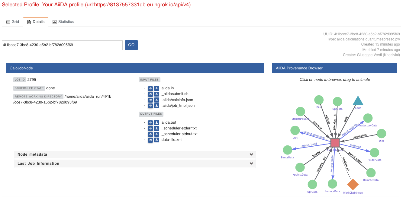
Fig. 1.5 The details view of the CalcJob node that created the original BandsData node.¶

You can check out here the details of the calculation, such as the input and output files, the Node metadata and Job information dropdown menus, etc. You may also want to know for which crystal structure the band structure was calculated. Although this information can also be found inside the input files, we will look for it directly in the input nodes, again by using the AiiDA Provenance Browser. This time we will look for the StructureData node (green circle) that has an outgoing link (so, the arrow points from the data node to the central current process node) with the label structure and click on it:

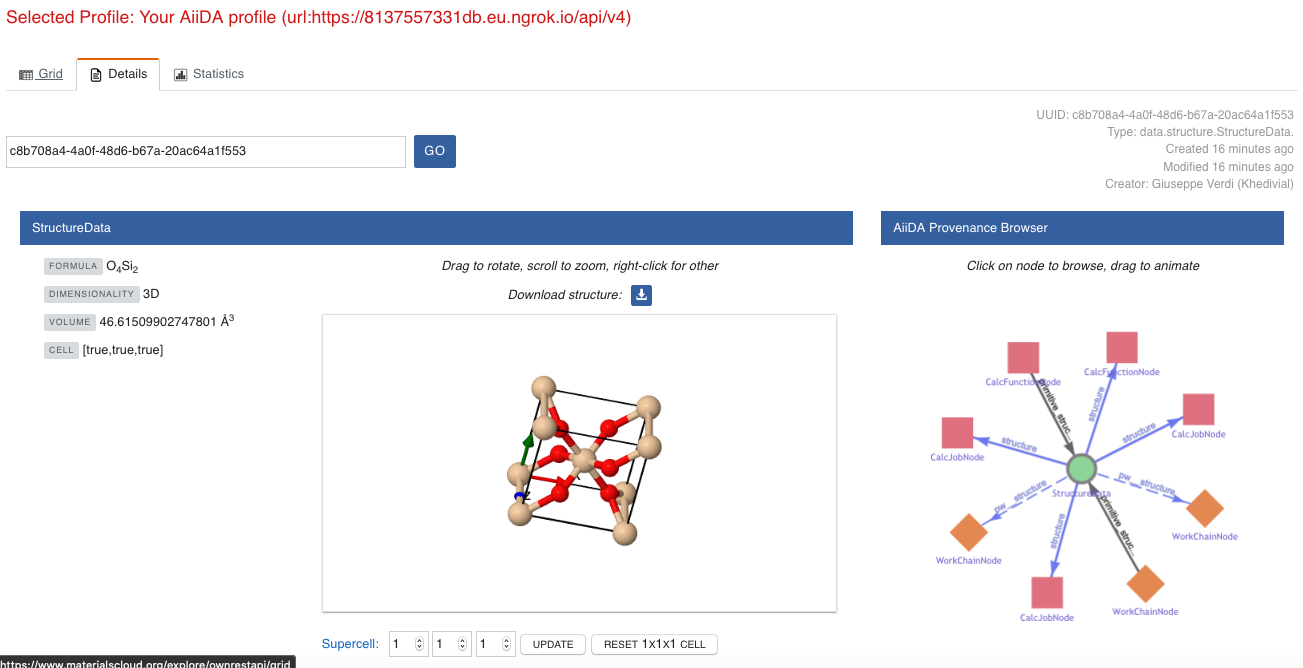
Fig. 1.6 The details view of the StructureData node that corresponds to the original BandsData node.¶

We can see in this particular case that the original BandsData corresponds to a Silica structure (your final structure might be different). You can look at the structure here, explore the details of the cell, etc.

Exercise: By now it is likely that your workflow has finished running. Repeat the same procedure described above to find the structure used to calculate the resulting band structure. You can identify this band structure easily as it will be the one with the newest creation time. Once you do:

Go to the details view for that BandsData node.

Look in the provenance browser for the calculation that created these bands and click on it.

Verify that this calculation is of type PwCalculation (look for the process_label in the node metadata subsection).

Look in the provenance browser for the StructureData that was used as input for this calculation.

As you can see, the explore tool of the Materials Cloud offers a very natural and intuitive interface to use for a light exploration of a database. However, you might already imagine that doing a more intensive kind of data mining of specific results this way can quickly become tedious. For this use cases, AiiDA has a more versatile tool: the QueryBuilder.

1.6. Finishing the workchain¶

Let’s stop ngrok using Ctrl+C and close its terminal, as well as stop the REST API (also using Ctrl+C). Let’s use verdi process show <PK> to inspect the PwBandsWorkChain and find the PK of its band_structure output. Instead of relying on the explore tool, we can also plot the band structure using the verdi shell:

$ verdi data bands export --format mpl_pdf --output band_structure.pdf <PK>

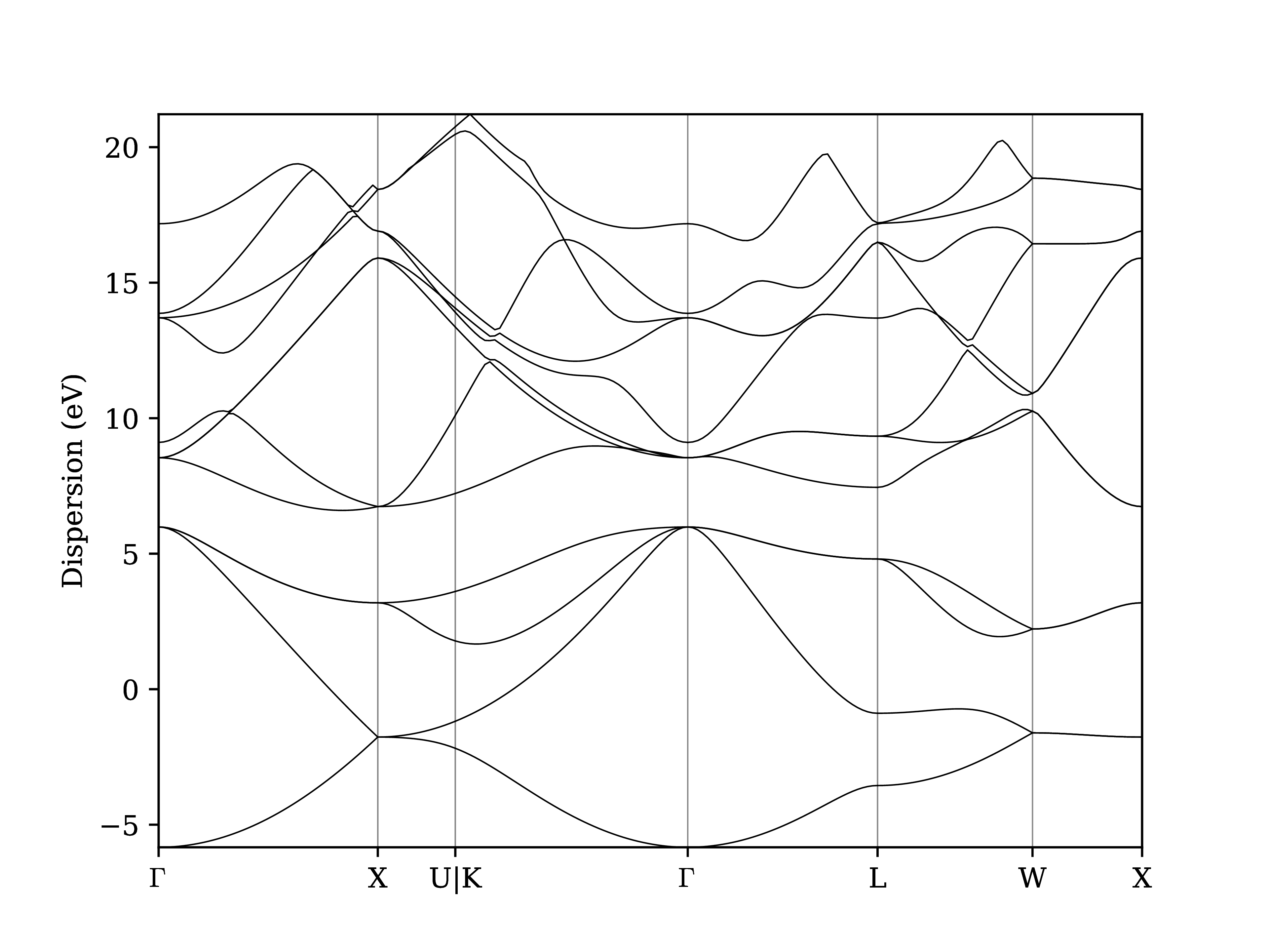
Fig. 1.7 Band structure computed by the PwBandStructureWorkChain.¶

Finally, the verdi process status command prints a hierarchical overview of the processes called by the work chain:

$ verdi process status 186
PwBandStructureWorkChain<186> Finished [0] [3:results]
    └── PwBandsWorkChain<201> Finished [0] [7:results]
        ├── PwRelaxWorkChain<203> Finished [0] [3:results]
        │   ├── PwBaseWorkChain<206> Finished [0] [7:results]
        │   │   ├── create_kpoints_from_distance<208> Finished [0]
        │   │   └── PwCalculation<212> Finished [0]
        │   └── PwBaseWorkChain<223> Finished [0] [7:results]
        │       ├── create_kpoints_from_distance<225> Finished [0]
        │       └── PwCalculation<229> Finished [0]
        ├── seekpath_structure_analysis<236> Finished [0]
        ├── PwBaseWorkChain<243> Finished [0] [7:results]
        │   ├── create_kpoints_from_distance<245> Finished [0]
        │   └── PwCalculation<249> Finished [0]
        └── PwBaseWorkChain<257> Finished [0] [7:results]
            └── PwCalculation<260> Finished [0]

The bracket [3:result] indicates the current step in the outline of the PwBandStructureWorkChain (step 3, with name result). The process status is particularly useful for debugging complex work chains, since it helps pinpoint where a problem occurred.

1.7. Querying the database¶

As you will use AiiDA to run your calculations, the database that stores all the data and the provenance will quickly grow to be very large. To help you find the needle that you might be looking for in this big haystack, we need an efficient search tool. AiiDA provides a tool to do exactly this: the QueryBuilder. The QueryBuilder acts as the gatekeeper to your database, to whom you can ask questions about its contents (also referred to as queries), by specifying what are looking for. In this final part of the tutorial, we will show an short demo on how to use the QueryBuilder to make these queries and understand/use the results.

First, we’ll import an archive of a study performed on a group of 57 different perovskites:

$ verdi import https://object.cscs.ch/v1/AUTH_b1d80408b3d340db9f03d373bbde5c1e/marvel-vms/tutorials/aiida_tutorial_2020_07_perovskites_v0.9.aiida

To help you organise your data, AiiDA allows you to group nodes together. Let’s have a look at the groups we’ve imported from the archive above, using the -C option so we also get a count of the number of nodes:

$ verdi group list --count
Info: to show groups of all types, use the `-a/--all` option.
  PK  Label            Type string    User               Node count
----  ---------------  -------------  ---------------  ------------
   5  tutorial_pbesol  core           aiida@localhost            57
   6  tutorial_lda     core           aiida@localhost            57
   7  tutorial_pbe     core           aiida@localhost            57

Each group contains a different set of 57 PwCalculation nodes (one for every different perovskite structure), organized according to the functional which was used in the calculation (LDA, PBE and PBEsol) . Imagine you want to use this data to understand the influence of the functional on the magnetization of the structure. Let’s build a query that helps us investigate this question. Start the verdi shell, and load the StructureData and PwCalculation classes:

In [1]: StructureData = DataFactory('structure')
   ...: PwCalculation = CalculationFactory('quantumespresso.pw')

We start every query by creating an instance of the QueryBuilder class:

In [2]: qb = QueryBuilder()

To build a query, we append entities (nodes, groups, …) to the query. Let’s build the query for one of the groups - say, tutorial_pbesol - step by step to help understand the process. We first append the Group to our QueryBuilder instance:

In [3]: qb.append(Group, filters={'label': 'tutorial_pbesol'}, tag='group');

Let’s explain the different arguments used in this call of the append() method:

The first positional argument is the Group class, preloaded in the verdi shell.

The first keyword argument is filters, here we filter for the group with label equal to tutorial_pbesol.

The second keyword argument is tag. This is a reference we will use to indicate relationships between nodes in future append() calls (as seen below).

Next, we’ll look for all the PwCalculations in this group:

In [4]: qb.append(PwCalculation, with_group='group', tag='pw');

Here, we use the 'group' tag we created in the previous step to query for PwCalculation’s in the tutorial_pbesol group using the with_group relationship argument. Moreover, we once again tag this append step of our query with pw. Let’s have a look at how many PwCalculation nodes we have in the tutorial_pbesol group:

In [5]: qb.count()
Out[5]: 57

Great, now let’s figure out which structures are magnetic! Of course, the information we are interested in are the structures and their absolute magnetization, which we’ll query for in the final two steps. First, we’ll append the StructureData to the query:

In [6]: qb.append(StructureData, with_outgoing='pw', project='extras.formula');

In this step, we’ve used the with_outgoing relationship to look for structures that have an outgoing link to the PwCalculations referenced with the pw tag. That means that from the PwCalculation’s perspective, the StructureData is an input. We also use the project keyword argument to project the formula of the structure, which has been conveniently stored in the extras of these StructureData nodes for the purpose of this tutorial. By projecting the formula, it will be a part of the results of our query. Try looking at the results of the current query using qb.all():

In [7]: qb.all()

The final append() call puts using relationships, filters and projections together. Here we are looking for the output_parameters Dict nodes, which are outputs of the PwCalculation nodes. However, we are only interested in structures for which the absolute_magnetization is larger than zero:

In [8]: qb.append(
   ...:     Dict, with_incoming='pw', filters={'attributes.absolute_magnetization': {'>': 0.0}},
   ...:     project='attributes.absolute_magnetization'
   ...: );

Let’s go over the arguments again:

The first positional argument tells the QueryBuilder we want to append Dict nodes to our query.

with_incoming indicates there is an incoming link from a PwCalculation, referenced by the 'pw' tag.

We’re filter-ing for magnetic structures, i.e. with absolute_magnetization above zero.

Finally, we project the absolute magnetization so it is added to the list of our results for each query result.

Our query is now complete! Let’s have a look at the results:

In [9]: qb.all()
Out[9]:
[['LaMnO3', 3.5],
 ['MnO3Sr', 3.15],
 ['CoO3Sr', 2.42],
 ['FeLaO3', 3.11],
 ['CoLaO3', 1.13],
 ['NiO3Sr', 0.77],
 ['FeO3Sr', 3.38]]

You can see that we’ve found 7 magnetic structures for the calculations in the tutorial_pbesol group, along with their formulas and magnetizations. We’ve set up a script (demo_query.py) that performs a similar query to obtain the magnetization and smearing energy for all results in the three groups, and then postprocess the data to visualize it. You can find it in the dropdown panel below:

Query demo script

from IPython.display import Image
from datetime import datetime, timedelta
import numpy as np
from matplotlib import gridspec, pyplot as plt

PwCalculation = CalculationFactory('quantumespresso.pw')
StructureData = DataFactory('structure')
KpointsData = DataFactory('array.kpoints')
Dict = DataFactory('dict')
UpfData = DataFactory('upf')

def plot_results(query_res):
    """
    :param query_res: The result of an instance of the QueryBuilder
    """
    smearing_unit_set,magnetization_unit_set,pseudo_family_set = set(), set(), set()
    # Storing results:
    results_dict = {}
    for pseudo_family, formula, smearing, smearing_units, mag, mag_units in query_res:
        if formula not in results_dict:
            results_dict[formula] = {}
        # Storing the results:
        results_dict[formula][pseudo_family] = (smearing, mag)
        # Adding to the unit set:
        smearing_unit_set.add(smearing_units)
        magnetization_unit_set.add(mag_units)
        pseudo_family_set.add(pseudo_family)

    # Sorting by formula:
    sorted_results = sorted(results_dict.items())
    formula_list = next(zip(*sorted_results))
    nr_of_results = len(formula_list)

    # Checks that I have not more than 3 pseudo families.
    # If more are needed, define more colors
    #pseudo_list = list(pseudo_family_set)
    if len(pseudo_family_set) > 3:
        raise Exception('I was expecting 3 or less pseudo families')

    colors = ['b', 'r', 'g']

    # Plotting:
    plt.clf()
    fig=plt.figure(figsize=(16, 9), facecolor='w', edgecolor=None)
    gs  = gridspec.GridSpec(2,1, hspace=0.01, left=0.1, right=0.94)

    # Defining barwidth
    barwidth = 1. / (len(pseudo_family_set)+1)
    offset = [-0.5+(0.5+n)*barwidth for n in range(len(pseudo_family_set))]
    # Axing labels with units:
    yaxis = ("Smearing energy [{}]".format(smearing_unit_set.pop()),
        "Total magnetization [{}]".format(magnetization_unit_set.pop()))
    # If more than one unit was specified, I will exit:
    if smearing_unit_set:
        raise ValueError('Found different units for smearing')
    if magnetization_unit_set:
        raise ValueError('Found different units for magnetization')

    # Making two plots, the top one for the smearing, the bottom one for the magnetization
    for index in range(2):
        ax=fig.add_subplot(gs[index])
        for i,pseudo_family in enumerate(pseudo_family_set):
            X = np.arange(nr_of_results)+offset[i]
            Y = np.array([thisres[1][pseudo_family][index] for thisres in sorted_results])
            ax.bar(X, Y,  width=0.2, facecolor=colors[i], edgecolor=colors[i], label=pseudo_family)
        ax.set_ylabel(yaxis[index], fontsize=14, labelpad=15*index+5)
        ax.set_xlim(-0.5, nr_of_results-0.5)
        ax.set_xticks(np.arange(nr_of_results))
        if index == 0:
            plt.setp(ax.get_yticklabels()[0], visible=False)
            ax.xaxis.tick_top()
            ax.legend(loc=3, prop={'size': 18})
        else:
            plt.setp(ax.get_yticklabels()[-1], visible=False)
        for i in range(0, nr_of_results, 2):
            ax.axvspan(i-0.5, i+0.5, facecolor='y', alpha=0.2)
        ax.set_xticklabels(list(formula_list),rotation=90, size=14, ha='center')
    plt.savefig('demo_query.pdf')


qb = QueryBuilder().append(
    Group, filters={'label':{'like':'tutorial_%'}}, project='label', tag='group'
).append(
    PwCalculation, tag='calculation', with_group='group'
).append(
    StructureData, project=['extras.formula'], tag='structure', with_outgoing='calculation'
).append(
    Dict, tag='results',
    project=['attributes.energy_smearing', 'attributes.energy_smearing_units',
             'attributes.total_magnetization', 'attributes.total_magnetization_units',
    ], with_incoming='calculation'
)

plot_results(qb.all())

Download it using wget:

$ wget https://aiida-tutorials.readthedocs.io/en/tutorial-2020-bigmap-lab/_downloads/6773ba4cad0c046e468d13e15186cdd8/demo_query.py

and use verdi run to execute it:

$ verdi run demo_query.py

The resulting plot should look like the one shown in Fig. 1.8.

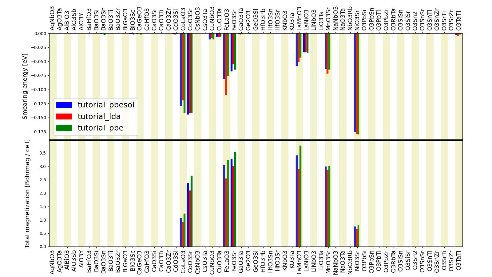
Fig. 1.8 Comparison of the absolute magnetization and smearing energy of the cell of the perovskite structures, calculated with different functionals.¶

1.8. What next?¶

You now have a first taste of the type of problems AiiDA tries to solve. Here are some options for how to continue:

Get a more detailed view of how to manipulate AiiDA objects in the extra section of this tutorial.
Continue with the in-depth tutorial.
Download the Quantum Mobile virtual machine and try running the tutorial on your laptop instead.
Try setting up AiiDA directly on your laptop.