2. Verdi command line
This part of the tutorial will help to familiarize you with the
command-line utility verdi, one of the most common ways to interact
with AiiDA. verdi with its subcommands enables a variety of
operations such as inspecting the status of ongoing or terminated
calculations, showing the details of calculations, computers, codes, or
data structures, access the input and the output of a calculation, etc.
Similar to the bash shell, verdi command support Tab completion. Try
right now to type verdi, followed by a space, in a terminal and tap
Tab twice to have a list of subcommands. Whenever you need the
explanation of a command type verdi help or add -h flag if you
are using any of the verdi subcommands. Finally, fields enclosed in
angular brackets, such as <pk>, are placeholders to be replaced by
the actual value of that field (an integer, a string, etc…).
2.1. The list of calculations
Let us try our first verdi commands. Type in the terminal
verdi calculation list
(Note: the first time you run this command, it might take a few seconds as it is the first time you are accessing the database in the virtual machine. Subsequent calls will be faster). This will print the list of ongoing calculations, which should be empty. The first output line should look like
PK    Creation    State    Type    Computer    Job state
----  ----------  -------  ------  ----------  -----------

Total results: 0

Info: last time an entry changed state: never
In order to print a list with all calculations that finished correctly
in the AiiDA database, you can use the -s/--states flag as follows:
verdi calculation list --states FINISHED
Another very typical option combination allows to get calculations in
any state (flag -a) generated in the past NUM days
(-p <NUM>): e.g., for calculation in the past 1 day:
verdi calculation list -p1 -a. Since you have not yet run any
calculations at the virtual machine that you currently use and all the
existing calculations were imported and belong to a different user, you
can type (flag -A shows the calculations of all the users):
verdi calculation list -A --states IMPORTED
Each row of the output identifies a calculation and shows some information about it. For a more detailed list of properties, choose one row by noting down its PK (primary key) number (first column of the output) and type in the terminal
verdi calculation show <pk>
The output depends on the specific pk chosen and should inform you about the input nodes (e.g. pseudopotentials, kpoints, initial structure, etc.), and output nodes (e.g. output structure, output parameters, etc.).
PKs/IDs vs. UUIDs: Beside the (integer) PK, very convenient to
reference a calculation or data node in your database, every node has a
UUID (Universally Unique ID) to identify it, that is preserved even when
you share some nodes with coworkers—while the PK will most likely
change. You can see the UUID in the output of verdi calculation show
or verdi node show. Moreover, if you have already a UUID and you
want to get the corresponding PK in your database, you can use
verdi node show -u <UUID>, as we are going to do now.
Let us now consider the node with
UUID = ce81c420-7751-48f6-af8e-eb7c6a30cec3, which identifies a
relaxation of a BaTiO(_3) unit cell run with Quantum Espresso pw.x.
You can check the information on this node and get the PK with:
$ verdi node show -u ce81c420-7751-48f6-af8e-eb7c6a30cec3
Property       Value
-------------  ------------------------------------
type           PwCalculation
pk             4235
uuid           ce81c420-7751-48f6-af8e-eb7c6a30cec3
label
description
ctime          2014-10-27 17:51:21.781045+00:00
mtime          2018-05-16 11:19:39.848446+00:00
process state
finish status
computer       [2] daint
code           pw-SVN-piz-daint

Inputs        PK  Type
----------  ----  -------------
parameters  4236  ParameterData
kpoints     4526  KpointsData
pseudo_Ba    966  UpfData
pseudo_Ti   4315  UpfData
settings    4529  ParameterData
pseudo_O    4342  UpfData
structure    436  StructureData

Outputs                    PK  Type
-----------------------  ----  -------------
output_kpoints           3665  KpointsData
output_parameters        3670  ParameterData
output_structure         3666  StructureData
retrieved                3668  FolderData
output_trajectory_array   265  ArrayData
remote_folder            1977  RemoteData
Keep in mind that you can also use just a part (beginning) of the UUID,
as long as it is unique, to show the node information information. For
example, to display the above information, you could also type
verdi node show -u ce81c420. In what follows, we are going to
mention only the prefixes of the UUIDs since they are sufficient to
identify the correct node.
2.2. A typical AiiDA graph
AiiDA stores inputs required by a calculation as well as the its outputs in the database. These objects are connected in a graph that looks like Fig. [fig:graph]. We suggest that you have a look to the figure before going ahead.
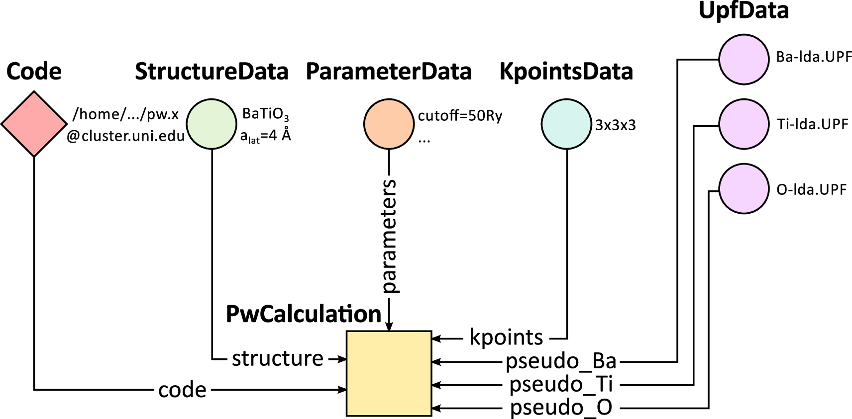
Fig. 2.27 Graph with all inputs (data, circles; and code, diamond) to the Quantum Espresso calculation (square) that you will create in Sec. [sec:qe] of this tutorial.
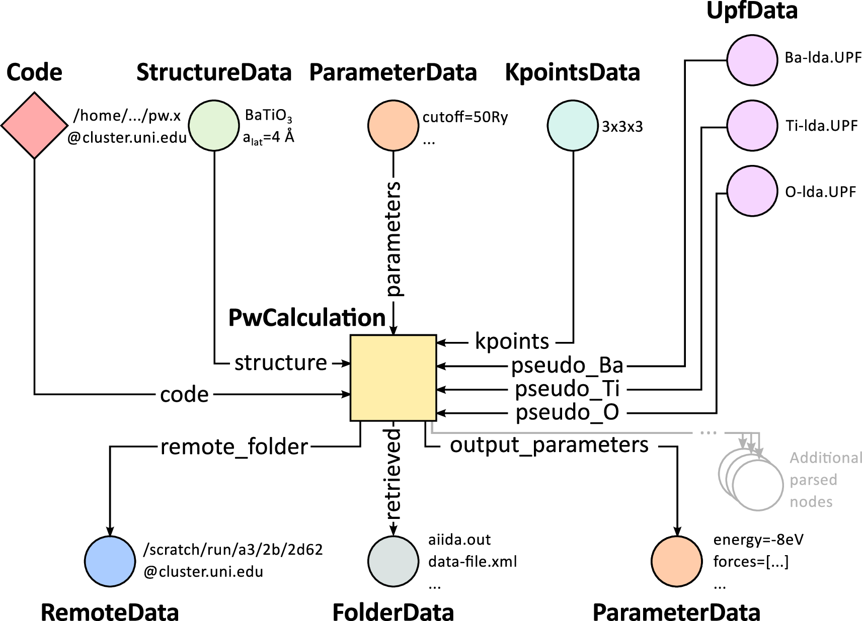
Fig. 2.28 Same as above, but also with the outputs that the daemon will create and connect automatically. The RemoteData node is created during submission and can be thought as a symbolic link to the remote folder in which the calculation runs on the cluster. The other nodes are created when the calculation has finished, after retrieval and parsing. The node with linkname “retrieved” contains the raw output files stored in the AiiDA repository; all other nodes are added by the parser. Additional nodes (symbolized in gray) can be added by the parser (e.g., an output StructureData if you performed a relaxation calculation, a TrajectoryData for molecular dynamics, …).
You can create a similar graph for any calculation node by using the
utility verdi graph generate <pk>. For example, before you obtained
information (in text form) for UUID = ce81c420. To visualize similar
information in graph(ical) form, run (replacing <pk> with the PK of
the node):
verdi graph generate <pk>
This command will create the file <pk>.dot that can be rendered by
means of the utility dot. If you now type
dot -Tpdf -o <pk>.pdf <pk>.dot
you will create a pdf file <pk>.pdf. You can open this file on the
Amazon machine by using evince or, if you feel that the ssh
connection is too slow, copy it via scp to your local machine. To do
so, if you are using Linux/Mac OS X, you can type in your local
machine:
scp aiidatutorial:<path_with_the_graph_pdf> <local_folder>
and then open the file. Alternatively, you can use graphical software to achieve the same, for instance: WinSCP on Windows, Cyberduck on the Mac, or the “Connect to server” option in the main menu after clicking on the desktop for Ubuntu.
Spend some time to familiarize yourself with the graph structure. Choose the root node (highlighted in blue) and trace back the parent calculation which produced the structure used as an input. This is an example of a Quantum ESPRESSO pw.x calculation, where the input structure was actually obtained as the output of a previous calculation. We will now inspect the different elements of this graph.
2.3. Inspecting the nodes of a graph
2.3.1. ParameterData and Calculations
Now, let us have a closer look at the some of the nodes appearing in the
graph. Choose the node of the type ParameterData with input link
name parameters (to double check, it should have UUID d1bbe1ea)
and type in the terminal:
verdi data parameter show <pk>
A ParameterData contains a dictionary (i.e., key–value pairs),
stored in the database in a format ready to be queried (we will learn
how to run queries later on in this tutorial). The command above will
print the content dictionary, containing the parameters used to define
the input file for the calculation. You can compare the dictionary with
the content of the raw input file to Quantum ESPRESSO (that was
generated by AiiDA) via the command
verdi calculation inputcat <pk>
where you substitute the pk of the calculation node. Check the consistency of the parameters written in the input file and those stored in the ParameterData node. Even if you don’t know the meaning of the input flags of a Quantum ESPRESSO calculation, you should be able to see how the input dictionary has been converted to Fortran namelists.
The previous command just printed the content of the “default” input
file aiida.in. To see a list of all the files used to run a
calculation (input file, submission script, etc.) instead type
verdi calculation inputls <pk>
(Adding a --color flag allows you to easily distinguish files from
folders by a different coloring).
Once you know the name of the file you want to visualize, you can call
the verdi calculation inputcat command specifying the path. For
instance, to see the submission script, you can do:
verdi calculation inputcat <pk> -p _aiidasubmit.sh
2.3.2. StructureData
Now let us focus on StructureData objects, representing a crystal
structure. We can consider for instance the input structure to the
calculation we were considering before (it should have UUID prefix
3a4b1270). Such objects can be inspected interactively by means of
an atomic viewer such as the one provided by ase. AiiDA however
supports several other viewers such as xcrysden, jmol, and
vmd. Type in the terminal
verdi data structure show --format ase <pk>
to show the selected structure (it will take a few seconds to appear,
and you can rotate the view with the right mouse button—if you receive
some errors, make sure you started your SSH connection with the -X
or -Y flag).
Alternatively, especially if showing them interactively is too slow over
SSH, you can export the content of a structure node in various popular
formats such as xyz or xsf. This is achieved by typing in the
terminal
verdi data structure export --format xsf <pk> > <pk>.xsf
You can open the generated xsf file and observe the cell and the
coordinates. Then, you can then copy <pk>.xsf from the Amazon
machine to your local one and then visualize it, e.g. with xcrysden (if
you have it installed):
xcrysden --xsf <pk>.xsf
2.3.3. Codes and computers
Let us focus now on the nodes of type code. A code represents (in
the database) the actual executable used to run the calculation. Find
the pk of such a node in the graph and type
verdi code show <pk>
The command prints information on the plugin used to interface the code to AiiDA, the remote machine on which the code is executed, the path of its executable, etc. To show a list of all available codes type
verdi code list
If you want to show all codes, including hidden ones and those created
by other users, use verdi code list -a -A. Now, among the entries of
the output you should also find the code just shown.
Similarly, the list of computers on which AiiDA can submit calculations is accessible by means of the command
verdi computer list -a
(-a shows all computers, also the one imported in your database but
that you did not configure, i.e., to which you don’t have access).
Details about each computer can be obtained by the command
verdi computer show <COMPUTERNAME>
Now you have the tools to answer the question:
What is the scheduler installed on the computer where the calculations of the graph have run?
2.3.4. Calculation results
The results of a calculation can be accessed directly from the calculation node. Type in the terminal
verdi calculation res <pk>
which will print the output dictionary of the “scalar” results parsed by AiiDA at the end of the calculation. Note that this is actually a shortcut for
verdi data parameter show <pk2>
where pk2 refers to the ParameterData node attached as an output of
the calculation node, with link name output_parameters.
By looking at the output of the command, what is the Fermi energy of the
calculation with UUID prefix ce81c420?
Similarly to what you did for the calculation inputs, you can access the output files via the commands
verdi calculation outputls <pk>
and
verdi calculation outputcat <pk>
Use the latter to verify that the Fermi energy that you have found in
the last step has been extracted correctly from the output file (Hint:
filter the lines containing the string “Fermi”, e.g. using grep, to
isolate the relevant lines).
The results of calculations are stored in two ways: ParameterData
objects are stored in the database, which makes querying them very
convenient, whereas ArrayData objects are stored on the disk. Once
more, use the command verdi data array show <pk> to know the Fermi
energy obtained from calculation with UUID prefix ce81c420 (you need
to use, this time, the PK of the output ArrayData of the calculation,
with link name output_trajectory_array). As you might have realized
the difference now is that the whole series of values of the Fermi
energy calculated after each relax/vc-relax step are stored. (The choice
of what to store in ParameterData and ArrayData nodes is made by
the parser of pw.x implemented in the aiida-quantumespresso
plugin.)
2.3.5. (Optional section) Comments
AiiDA offers the possibility to attach comments to a calculation node, in order to be able to remember more easily its details. Node with UUID prefix ce81c420 has no comment already defined, but you can add a very instructive one by typing in the terminal
verdi comment add -c "vc-relax of a BaTiO3 done with QE pw.x" <pk>
Now, if you ask for a list of all comments associated to that calculation by typing
verdi comment show <pk>
the comment that you just added will appear together with some useful
information such as its creator and creation date. We let you play with
the other options of verdi comment command to learn how to update or
remove comments.
2.4. AiiDA groups of calculations
In AiiDA, calculations (and more generally nodes) can be organized in groups, which are particularly useful to assign a set of calculations or data to a common project. This allows you to have quick access to a whole set of calculations with no need for tedious browsing of the database or writing complex scripts for retrieving the desired nodes. Type in the terminal
verdi group list
to show a list of the groups that already exist in the database. Choose
the PK of the group named tutorial_pbesol and look at the
calculations that it contains by typing
verdi group show <pk>
In this case, we have used the name of the group to organize calculations according to the pseudopotential that has been used to perform them. Among the rows printed by the last command you will be able to find the calculation we have been inspecting until now.
If, instead, you want to know all the groups to which a specific node belomngs, you can run
verdi group list --node <pk>