These appendices consist of optional exercises, and are mentioned in earlier parts of the tutorial. Go through them only if you have time.

5. More workflow logic: while loops and conditional statements

In the previous sections, you have been introduced to WorkChains, and the reason for using them over ‘standard’ work functions. However, in the original example, the spec.outline was quite simple, with a ‘static’ sequence of two steps. Most often, however, you need dynamic workflows, where you need to decide at runtime whether to continue to compute or not (e.g. in a convergence loop, where you need to stop if convergence has been achieved). To support this scenario, the spec.outline can support logic: while loops and if/elif/else blocks. The simplest way to explain it is to show an example:

from aiida.engine import if_, while_

spec.outline(
    cls.s1,
    if_(cls.isA)(
        cls.s2
    ).elif_(cls.isB)(
        cls.s3
    ).else_(
        cls.s4
    ),
    cls.s5,
    while_(cls.condition)(
        cls.s6
    ),
)

that would roughly correspond, in a python syntax, to:

s1()
if isA():
    s2()
elif isB():
    s3()
else:
    s4()
s5()
while condition():
    s6()

The only constraint is that condition functions (in the example above isA, isB and condition) must be class methods that returns True or False depending on whether the condition is met or not.

A suggestion on how to write new workchains: use the outline to help you in designing the logic. First create the spec outline writing, almost if you were explaining it in words, what you expect the workflow to do. Then, define one by one the methods.

5.1. Pressure convergence

For example, we have prepared a simple workflow (using work chains, work functions and calculation functions) to optimize the lattice parameter of silicon efficiently using Newton’s algorithm on the energy derivative, i.e. the pressure \(p=-dE/dV\). You can download this code here The outline looks like this:

spec.outline(
    cls.setup,
    cls.put_step0_in_ctx,
    cls.move_next_step,
    while_(cls.not_converged)(
        cls.move_next_step,
    ),
    cls.finish
)

This outline already roughly explains the algorithm: after an initialization (setup) and putting the first step (number zero) in the ctx (put_step0_in_ctx), a function to move to the next step is called (move_next_step). This is iterated while a given convergence criterion is not met (not_converged). Finally, some reporting is done, including returning some output nodes (finish).

If you are interested in the details of the algorithm, you can inspect the file. The main ideas are described here:

setup Generate a pw.x calculation for the input structure (with volume (V)), and one for a structure where the volume is \(V+4 \mbox{\normalfont\AA}^3\) (just to get a closeby volume). Store the results in the context as r0 and r1

put_step0_in_ctx Store in the context \(V\), \(E(V)\) and \(dE/dV\) for the first calculation r0

move_next_step This is the most important function. Calculate \(V\), \(E(V)\) and \(dE/dV\) for r1. Also, estimate \(d^2E/dV^2\) from the finite difference of the first derivative of r0 and r1 (helper functions to achieve this are provided). Get the \(a\), \(b\) and \(c\) coefficients of a parabolic fit \(E = aV^2 + bV + c\) and estimate the expected minimum of the EOS function as the minimum of the fit \(V_0 = -b / 2a\). Finally, replace r0 with r1 in the context (i.e., get rid of the oldest point) and launch a new pw calculation at volume \(V_0\), that will be stored in the context replacing r1. In this way, at the next iteration r0 and r1 will contain the latest two simulations. Finally, at each step some relevant information (coefficients \(a\), \(b\) and \(c\), volumes, energies, energy derivatives, …) are stored in a list called steps. This whole list is stored in the context because it provides quantities to be preserved between different work chain steps.

not_converged Return True if convergence has not been achieved yet. Convergence is achieved if the difference in volume between the two latest simulations is smaller than a given threshold volume_tolerance.

finish This is the final step. Mainly, we return the output nodes: steps with the list of results at each step, and structure with the final converged structure.

The results returned in steps can be used to represent the evolution of the minimisation algorithm. A possible way to visualize it is presented in Fig. 5.6 obtained with an initial lattice constant of alat = 5.2.

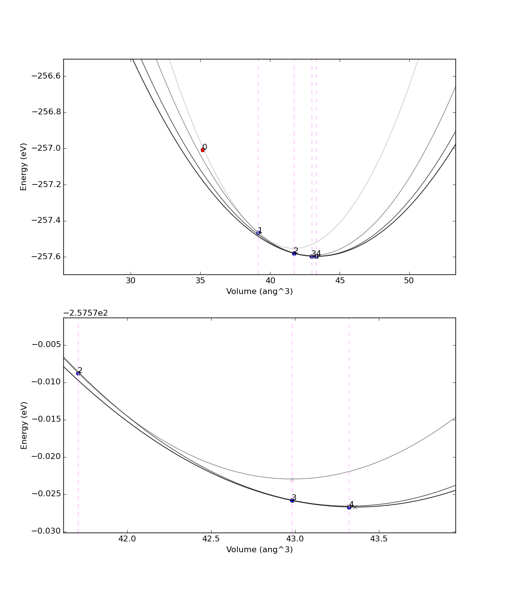
Fig. 5.5 Example of results of the convergence algorithm presented in this section. The bottom plot is a zoom near the minimum. The dots represent the (volume,energy) points obtained from Quantum ESPRESSO, and the numbers indicate at which iteration they were obtained. The parabolas represent the parabolic fits used in the algorithm; the minimum of the parabola is represented with a small cross, in correspondence of the vertical lines, used as the volume for the following step.