AiiDA basics
Contents
AiiDA basics
This module will give you a first taste of some of the features of AiiDA, and help familiarize you with the verdi command-line interface (CLI), as well as AiiDA’s IPython shell.
Tip
The verdi command supports tab-completion!
In the terminal, type verdi, followed by a space and press the ‘Tab’ key twice to show a list of all the available sub commands.
Next, try typing verdi st and then press “Tab” again.
This should tab-complete into verdi status.
For help on verdi or any of its subcommands, simply append the --help/-h flag, e.g.:
$ verdi status -h
![]() Further reading
Further reading
More details on the verdi CLI can be found in the AiiDA documentation.
Provenance
To start, we need to briefly introduce one of the most important concepts in AiiDA: provenance. An AiiDA database does not only contain the results of your calculations, but also their inputs and each step that was executed to obtain them. All of this information is stored in the form of a directed acyclic graph (DAG). As an example, Fig. 1 shows the provenance of the calculations of the first part of this tutorial.
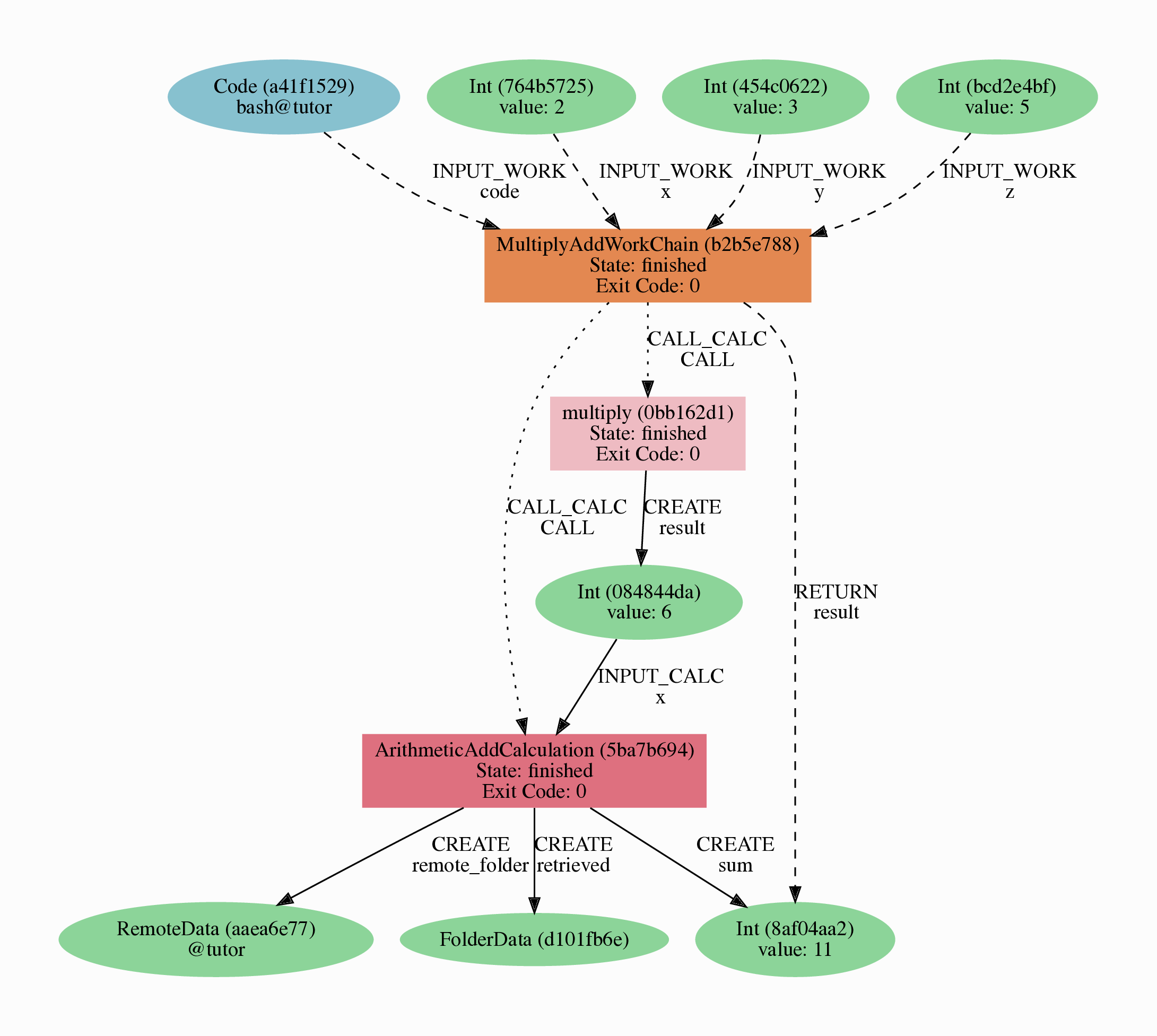
Fig. 1 Provenance Graph of a basic AiiDA WorkChain.
In the provenance graph, you can see different types of nodes represented by different shapes.
The green ellipses are Data nodes, the blue ellipse is a Code node, and the rectangles represent processes, i.e. the calculations performed in your workflow.
The provenance graph allows us to not only see what data we have, but also how it was produced. During this basic tutorial we will first be using AiiDA to generate the provenance graph in Fig. 1, step by step.
Data nodes
Before running any calculations, let’s create and store a data node. AiiDA ships with an interactive IPython shell that has many basic AiiDA classes pre-loaded. To start the IPython shell, simply type in the terminal:
$ verdi shell
 Variables
Variables are a basic concept in Python and most programming languages. Understanding them is essential, so in case you are unfamiliar you can find a very short introduction here.
AiiDA implements data node types for the most common types of data (int, float, str, etc.), which you can extend with your own (composite) data node types if needed.
For this tutorial, we’ll keep it very simple, and start by initializing an Int node and assigning it to the node variable:
In [1]: node = Int(2)
Tip
Commands you have to execute in the bash terminal or the verdi shell can be clearly distinguished via the corresponding prompts:
Bash terminal:
$ I am a bash command!verdi shell:In [1]: I am a verdi shell command
There is also a copy button in the top right of each code-snippet, that will only copy the input. Try this with the code snippet after this tip!
We can check the contents of the node variable like this:
In [2]: node
Out[2]: <Int: uuid: eac48d2b-ae20-438b-aeab-2d02b69eb6a8 (unstored) value: 2>
Quite a bit of information on our freshly created node is returned:
The data node is of the type
IntThe node has the universally unique identifier (UUID)
eac48d2b-ae20-438b-aeab-2d02b69eb6a8The node is currently not stored in the database
(unstored)The integer value of the node is
2
Let’s store the node in the database:
In [3]: node.store()
Out[3]: <Int: uuid: eac48d2b-ae20-438b-aeab-2d02b69eb6a8 (pk: 1) value: 2>
As you can see, the data node has now been assigned a primary key (PK), a number that identifies the node in your database (pk: 1).
The PK and UUID both reference the node with the only difference that the PK is unique for your local database only, whereas the UUID is a globally unique identifier and can therefore be used between different databases.
You’ll typically use the PK when you are working within a single database and the UUID when you are collaborating with others to refer to nodes in other databases.
Important
It is very likely that the PKs shown in the examples will be different for your database! The UUIDs are generated randomly and are therefore guaranteed to be different for nodes created during the tutorial.
Next, let’s leave the IPython shell by typing exit() and then enter.
Back in the terminal, use the verdi command line interface (CLI) to check the data node we have just created:
$ verdi node show <PK>
This prints something like the following:
Property     Value
-----------  ------------------------------------
type         Int
pk           1
uuid         eac48d2b-ae20-438b-aeab-2d02b69eb6a8
label
description
ctime        2020-05-13 08:58:15.193421+00:00
mtime        2020-05-13 08:58:40.976821+00:00
![]() Further reading
Further reading
AiiDA already provides many standard data types, but you can also create your own.
Once again, we can see that the node is of type Int, has PK = 1, and UUID = eac48d2b-ae20-438b-aeab-2d02b69eb6a8.
Besides this information, the verdi node show command also shows the (empty) label and description, as well as the time the node was created (ctime) and last modified (mtime).
Calculation functions
Once your data is stored in the database, it is ready to be used for some computational task.
For example, let’s say you want to multiply two Int data nodes.
The following Python function:
def multiply(x, y):
    return x * y
Decorators
A decorator can be used to add functionality to an existing function. You can read more about them here.
will give the desired result when applied to two Int nodes, but the calculation will not be stored in the provenance graph.
However, we can use a Python decorator provided by AiiDA to automatically make it part of the provenance graph.
Start up the AiiDA IPython shell again using verdi shell and execute the following code snippet:
In [1]: from aiida.engine import calcfunction
   ...:
   ...: @calcfunction
   ...: def multiply(x, y):
   ...:     return x * y
This converts the multiply function into an AiIDA calculation function, the most basic execution unit in AiiDA.
Next, load the Int node you have created in the previous section using the load_node function and the PK of the data node:
In [2]: x = load_node(pk=<PK>)
Of course, we need another integer to multiply with the first one.
Let’s create a new Int data node and assign it to the variable y:
In [3]: y = Int(3)
Now it’s time to multiply the two numbers!
In [4]: multiply(x, y)
Out[4]: <Int: uuid: 42541d38-1fb3-4f60-8122-ab8b3e723c2e (pk: 4) value: 6>
Success!
The calcfunction-decorated multiply function has multiplied the two Int data nodes and returned a new Int data node whose value is the product of the two input nodes.
Note that by executing the multiply function, all input and output nodes are automatically stored in the database:
In [5]: y
Out[5]: <Int: uuid: 7865c8ff-f243-4443-9233-dd303a9be3c5 (pk: 2) value: 3>
We had not yet stored the data node assigned to the y variable, but by providing it as an input argument to the multiply function, it was automatically stored with PK = 2.
Similarly, the returned Int node with value 6 has been stored with PK = 4.
Let’s once again leave the IPython shell with exit() and look for the process we have just run using the verdi CLI:
$ verdi process list
The returned list will be empty, but don’t worry!
By default, verdi process list only returns the active processes.
If you want to see all processes (i.e. also the processes that are terminated), simply add the -a/--all option:
$ verdi process list -a
You should now see something like the following output:
  PK  Created    Process label    Process State    Process status
----  ---------  ---------------  ---------------  ----------------
   3  1m ago     multiply         ⏹ Finished [0]

Total results: 1

Info: last time an entry changed state: 1m ago (at 09:01:05 on 2020-05-13)
We can see that our multiply calcfunction was created 1 minute ago, assigned the PK 3, and has Finished.
As a final step, let’s have a look at the provenance of this simple calculation.
The provenance graph can be automatically generated using the verdi CLI.
Let’s generate the provenance graph for the multiply calculation function we have just run with PK = 3:
$ verdi node graph generate <PK>
The command will write the provenance graph to a .pdf file.
The name of said file will start with the PK of your calculation node and have an intermediate .dot extension (in this case it would be 3.dot.pdf).
The result should look something like the graph shown in Fig. 2.
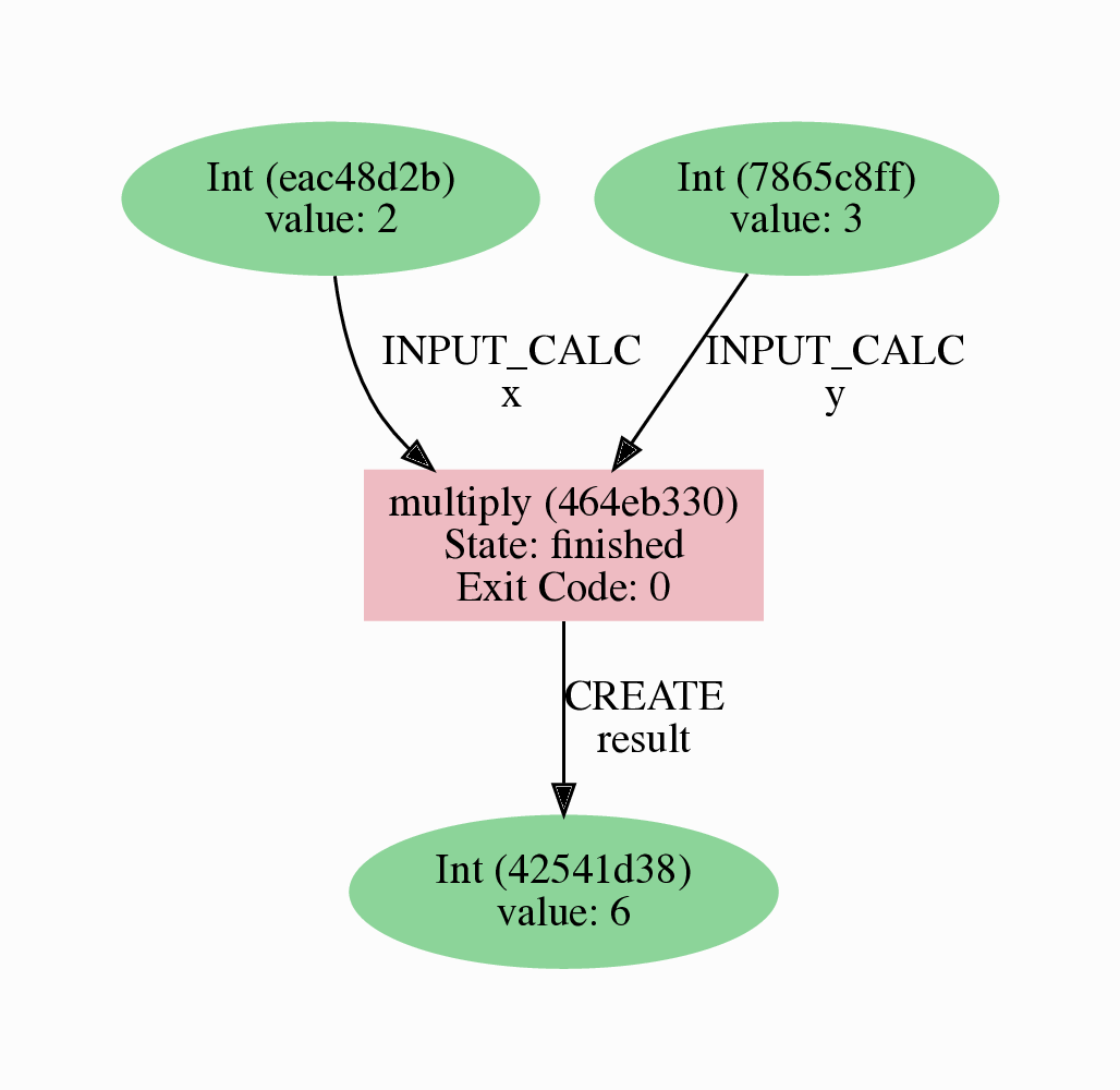
Fig. 2 Provenance graph of the multiply calculation function.
CalcJobs
When running calculations that require a (possibly non-Python) code external to AiiDA and/or run on a remote machine, a simple calculation function is no longer sufficient.
For this purpose, AiiDA provides the CalcJob process class.
To see all calculations available from the AiiDA packages installed in your environment you can use the verdi plugin command:
$ verdi plugin list aiida.calculations
This will show you a long list of entry points: strings that are used to identify each plugin within AiiDA.
In this list you should be able to see the arithmetic.add entry point, which identifies the calculation job we want to run:
Registered entry points for aiida.calculations:
(...)
* arithmetic.add
(...)

Info: Pass the entry point as an argument to display detailed information
Note
If you just run verdi plugin list, you will get a list of all possible plugin groups.
To get more information about the inputs, outputs, etc. of this calculation job, just follow the instructions at the end of the output and pass the arithmetic.add entry point as an additional argument for the command:
$ verdi plugin list aiida.calculations arithmetic.add
There is a lot of information we obtain with this command:
Description:

	`CalcJob` implementation to add two numbers using bash for testing and demonstration purposes.

Inputs:
           code:  required  Code             The `Code` to use for this job.
              x:  required  Int, Float       The left operand.
              y:  required  Int, Float       The right operand.
       metadata:  optional
Outputs:
  remote_folder:  required  RemoteData       Input files necessary to run the process will be stored in this folder node ...
      retrieved:  required  FolderData       Files that are retrieved by the daemon will be stored in this node. By defa ...
            sum:  required  Int, Float       The sum of the left and right operand.
   remote_stash:  optional  RemoteStashData  Contents of the `stash.source_list` option are stored in this remote folder ...
Exit codes:
              1:  The process has failed with an unspecified error.
              2:  The process failed with legacy failure mode.
             11:  The process did not register a required output.
            100:  The process did not have the required `retrieved` output.
            110:  The job ran out of memory.
            120:  The job ran out of walltime.
            310:  The output file could not be read.
            320:  The output file contains invalid output.
            410:  The sum of the operands is a negative number.
The first is description of the calculation, which explains that it adds two numbers together.
Then there are the inputs, of which 3 are required: the code to be used to add the numbers up, and the two numbers (x and y) to add.
Finally, note the sum among the outputs, which contains the result of the addition.
Now that we understand what our CalcJob does and what it needs, let’s see what we need to do to run it.
Preliminary setup
Before you run a CalcJob, you need to have two things: a code to run the desired calculation and a computer for the calculation to run on.
Most of our tutorial environments already have the localhost computer set up.
You can check that this is the case with verdi computer list:
$ verdi computer list
Info: List of configured computers
Info: Use 'verdi computer show COMPUTERLABEL' to display more detailed information
* localhost
If not, you can find instructions on how to do so in the dropdown below.
Setting up the localhost computer
You can set up the computer using the verdi computer subcommand:
$ verdi computer setup -L localhost -H localhost -T local -S direct -w `echo $HOME/aiida_run` --mpiprocs-per-machine 1 -n
$ verdi computer configure local localhost --safe-interval 5 -n
The first commands sets up the computer with the following options:
label (
-L): localhosthostname (
-H): localhosttransport (
-T): localscheduler (
-S): directwork-dir (
-w): Theaiida_runsubdirectory of the home directory--mpiprocs-per-machine: The default number of MPI processes per machine is set to 1.
The second command configures the computer with a minimum interval between connections (--safe-interval) of 5 seconds.
For both commands, the non-interactive option (-n) is added to not prompt for extra input.
Next, let’s set up the code we’re going to use for the tutorial:
$ verdi code setup -L add --on-computer --computer=localhost -P arithmetic.add --remote-abs-path=/bin/bash -n
This command sets up a code with label add on the computer localhost, using the plugin arithmetic.add.
A typical real-world example of a computer is a remote supercomputing facility. Codes can be anything from a Python script to powerful ab initio codes such as Quantum ESPRESSO or machine learning tools like Tensorflow. Let’s have a look at the codes that are available to us:
$ verdi code list
# List of configured codes:
# (use 'verdi code show CODEID' to see the details)
(...)
* pk 1 - add@localhost
In the output above you can see a the code add@localhost, with PK = 1, in the printed list.
Again, in your output you may have other codes listed or a different PK depending on your specific setup, but you should still be able to identify the code by its label.
The add@localhost identifier indicates that the code with label add is run on the computer with label localhost.
To see more details about the computer, you can use the following verdi command:
$ verdi computer show localhost
Computer name:     localhost
--------------  ------------------------------------
Label           localhost
PK              1
UUID            b7ea4398-3c05-4a43-9214-9c4d91d40c8f
Description     this computer
Hostname        localhost
Transport type  local
Scheduler type  direct
Work directory  /home/aiida/aiida_run/
Shebang         #!/bin/bash
Mpirun command  mpirun -np {tot_num_mpiprocs}
Prepend text
Append text
--------------  ------------------------------------
We can see that the Work directory has been set up as the aiida_run subdirectory of the home directory.
This is the directory in which the calculations running on the localhost computer will be executed.
Note
You may have noticed that in our example, the PK of the localhost computer is 1, same as the Int node we created at the start of this tutorial.
This is because different entities, such as nodes, computers and groups, are stored in different tables of the database.
So, the PKs for each entity type are unique for each database, but entities of different types can have the same PK within one database.
Running the CalcJob
Let’s now start up the verdi shell again and load the arithmetic.add calculations using the CalculationFactory:
In [1]: ArithmeticAdd = CalculationFactory('arithmetic.add')
Now you need to gather the actual nodes that will be used as inputs for the calculation. If you remember from before, there are three inputs we need to define:
code (the
Codeto use for the job)x (the left operand, of type
IntorFloat)y (the right operand, of type
IntorFloat)
For the code, you will use the add@localhost code using its label:
In [2]: code = load_code(label='add@localhost')
Let’s use the Int node that was created by our previous calcfunction as one of the inputs and a new node as the second input:
In [3]: x = load_node(pk=<PK>)
   ...: y = Int(5)
Tip
In case you don’t remember the PK of the output node from the previous calculation, check the provenance graph you generated earlier and use the UUID of the output node instead. For example (remember that your UUID is guaranteed to be different!):
In [3]: x = load_node(uuid='42541d38')
   ...: y = Int(5)
Note that you don’t have to provide the entire UUID to load the node. As long as the first part of the UUID is unique within your database, AiiDA will find the node you are looking for.
To execute the CalcJob, you need to feed it (together with the inputs) to the run function provided by the AiiDA engine:
In [4]: from aiida.engine import run
   ...: run(ArithmeticAdd, code=code, x=x, y=y)
Wait for the process to complete, as it may take a couple of seconds. Once it is done, it will return a dictionary with the output nodes:
Out[4]:
{'sum': <Int: uuid: 7d5d781e-8f17-498a-b3d5-dbbd3488b935 (pk: 8) value: 11>,
'remote_folder': <RemoteData: uuid: 888d654a-65fb-4da0-b3bc-d63f0374f274 (pk: 9)>,
'retrieved': <FolderData: uuid: 4733aa78-2e2f-4aeb-8e09-c5cfb58553db (pk: 10)>}
Besides the sum of the two Int nodes, the calculation function also returns two other outputs: one of type RemoteData and one of type FolderData.
See the topics section on calculation jobs for more details.
Now, exit the IPython shell and once more check for all processes:
$ verdi process list -a
You should now see two processes in the list.
One is the multiply calcfunction you ran earlier, the second is the ArithmeticAddCalculation CalcJob that you have just run.
Grab the PK of the ArithmeticAddCalculation, and generate the provenance graph.
The result should look like the graph shown in Fig. 3.
$ verdi node graph generate <PK>
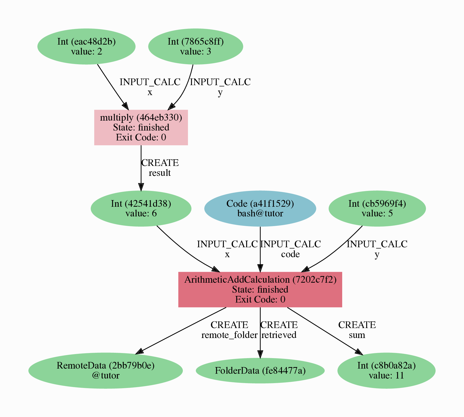
Fig. 3 Provenance graph of the ArithmeticAddCalculation CalcJob, with one input provided by the output of the multiply calculation function.
You can see more details on any process, including its inputs and outputs, using the verdi shell:
$ verdi process show <PK>
Submitting to the daemon
When we used the run command in the previous section, the IPython shell was blocked while it was waiting for the CalcJob to finish.
This is not a problem when we’re simply multiplying two numbers, but if we want to run multiple calculations that take hours or days, this is no longer practical.
Instead, we are going to submit the CalcJob to the AiiDA daemon.
The daemon is a program that runs in the background and manages submitted calculations until they are terminated.
Let’s first check the status of the daemon using the verdi CLI:
$ verdi daemon status
If the daemon is running, the output will be something like the following:
Profile: tutorial
Daemon is running as PID 96447 since 2020-05-22 18:04:39
Active workers [1]:
  PID    MEM %    CPU %  started
-----  -------  -------  -------------------
96448    0.507        0  2020-05-22 18:04:39
Use verdi daemon [incr | decr] [num] to increase / decrease the amount of workers
In this case, let’s stop it for now:
$ verdi daemon stop
Next, let’s submit the CalcJob we ran previously.
Start the verdi shell and execute the Python code snippet below.
This follows all the steps we did previously, but now uses the submit function instead of run:
In [1]: from aiida.engine import submit
   ...:
   ...: ArithmeticAdd = CalculationFactory('arithmetic.add')
   ...: code = load_code(label='add@localhost')
   ...: x = load_node(pk=<PK>)
   ...: y = Int(5)
   ...:
   ...: submit(ArithmeticAdd, code=code, x=x, y=y)
When using submit the calculation job is not run in the local interpreter but is sent off to the daemon and you get back control instantly.
Instead of the result of the calculation, it returns the node of the CalcJob that was just submitted:
Out[1]: <CalcJobNode: uuid: e221cf69-5027-4bb4-a3c9-e649b435393b (pk: 12) (aiida.calculations:arithmetic.add)>
Let’s exit the IPython shell and have a look at the process list:
$ verdi process list
You should see the CalcJob you have just submitted, with the state Created:
  PK  Created    Process label             Process State    Process status
----  ---------  ------------------------  ---------------  ----------------
  12  13s ago    ArithmeticAddCalculation  ⏹ Created

Total results: 1

Info: last time an entry changed state: 13s ago (at 09:06:57 on 2020-05-13)
Warning: the daemon is not running
The CalcJob process is now waiting to be picked up by a daemon runner, but the daemon is currently disabled.
Let’s start it up (again):
$ verdi daemon start
Now you can either use verdi process list to follow the execution of the CalcJob.
Let’s wait for the CalcJob to complete (state changes to “Finished”).
Use verdi process list -a to see all processes we have run so far:
  PK  Created    Process label             Process State    Process status
----  ---------  ------------------------  ---------------  ----------------
   3  6m ago     multiply                  ⏹ Finished [0]
   7  2m ago     ArithmeticAddCalculation  ⏹ Finished [0]
  12  1m ago     ArithmeticAddCalculation  ⏹ Finished [0]

Total results: 3

Info: last time an entry changed state: 14s ago (at 09:07:45 on 2020-05-13)
Workflows
So far we have executed each process manually.
AiiDA allows us to automate these steps by linking them together in a workflow, whose provenance is stored to ensure reproducibility.
For this tutorial we have prepared a basic WorkChain that is already implemented in aiida-core.
You will see more details on how to write such a work chain in the module on writing work chains.
Note
Besides work chains, workflows can also be implemented as work functions. These are ideal for workflows that are not very computationally intensive and can be easily implemented in a Python function.
Just like we did for aiida.calculations, to see all available workflows you can run verdi plugin list aiida.workflows.
You should be able to see the arithmetic.multiply_add entry point, among others.
Once again, to get the specific information for this work chain you just need to run:
$ verdi plugin list aiida.workflows arithmetic.multiply_add
Which gives the following information on the work chain:
Description:

	WorkChain to multiply two numbers and add a third, for testing and demonstration purposes.

Inputs:
      code:  required  Code
         x:  required  Int
         y:  required  Int
         z:  required  Int
  metadata:  optional
Outputs:
    result:  required  Int
Exit codes:
         1:  The process has failed with an unspecified error.
         2:  The process failed with legacy failure mode.
        10:  The process returned an invalid output.
        11:  The process did not register a required output.
       400:  The result is a negative number.
Let’s run the WorkChain above!
Just as we did before with the CalculationFactory, we will load the MultiplyAddWorkChain using the WorkflowFactory (which works in the same way but is used for workflows instead of calculations).
Start up the verdi shell and run:
In [1]: MultiplyAddWorkChain = WorkflowFactory('arithmetic.multiply_add')
We will now load the necessary nodes for each of the inputs required by the WorkChain (see the specifications above):
In [2]: code = load_code(label='add@localhost')
   ...: x = Int(2)
   ...: y = Int(3)
   ...: z = Int(5)
And finally we will submit it to the daemon using the submit function from the AiiDA engine:
In [3]: from aiida.engine import submit
   ...: submit(MultiplyAddWorkChain, code=code, x=x, y=y, z=z)
Now quickly leave the IPython shell and check the process list:
$ verdi process list -a
Depending on which step the workflow is running, you should get something like the following:
  PK  Created    Process label             Process State    Process status
----  ---------  ------------------------  ---------------  ------------------------------------
   3  7m ago     multiply                  ⏹ Finished [0]
   7  3m ago     ArithmeticAddCalculation  ⏹ Finished [0]
  12  2m ago     ArithmeticAddCalculation  ⏹ Finished [0]
  19  16s ago    MultiplyAddWorkChain      ⏵ Waiting        Waiting for child processes: 22
  20  16s ago    multiply                  ⏹ Finished [0]
  22  15s ago    ArithmeticAddCalculation  ⏵ Waiting        Waiting for transport task: retrieve

Total results: 6

Info: last time an entry changed state: 0s ago (at 09:08:59 on 2020-05-13)
We can see that the MultiplyAddWorkChain is currently waiting for its child process, the ArithmeticAddCalculation, to finish.
Check the process list again for all processes (You should know how by now!).
After about half a minute, all the processes should be in the Finished state.
We can now generate the full provenance graph for the WorkChain using the <PK> of the MultiplyAddWorkChain:
$ verdi node graph generate <PK>
Open the generated pdf file. Look familiar? The provenance graph should be similar to the one we showed at the start of this tutorial (Fig. 4).
Fig. 4 Final provenance Graph of the basic AiiDA tutorial.
Next steps
Congratulations! You have completed the first step to becoming an AiiDA expert.
The next step is to learn all about running processes with AiiDA.