2. AiiDA basics¶

This part of the tutorial will give you a first taste of some of the features of AiiDA, and help you familiarize with the verdi command-line interface (CLI), as well as AiiDA’s IPython shell.

Important

Before starting this tutorial, make sure you have watched the demonstration on working with your virtual machine. Also remember to run workon aiida in any new terminal, in order to enter the correct virtual environment, otherwise the verdi command will not be available.

The verdi command supports tab-completion: In the terminal, type verdi, followed by a space and press the ‘Tab’ key twice to show a list of all the available sub commands.
For help on verdi or any of its subcommands, simply append the --help/-h flag, e.g.:
```
$ verdi quicksetup -h
```

More details on verdi can be found in the online documentation.

2.1. Setting up a profile¶

After installing AiiDA, the first step is to create a “profile”. Typically, you would be using one profile per independent research project.

The easiest way of setting up a new profile is through verdi quicksetup. Let’s set up a new profile that we will use throughout this tutorial:

$ verdi quicksetup

This will prompt you for some information, such as the name of the profile, your name, etc. The information about you as a user will be associated with all the data that you create in AiiDA and it is important for attribution when you will later share your data with others. After you have answered all the questions, a new profile will be created, along with the required database and repository.

Note

verdi quicksetup is a user-friendly wrapper around the verdi setup command that provides more control over the profile setup. As explained in the documentation, verdi setup expects certain external resources (such as the database and RabbitMQ) to already have been pre-configured. verdi quicksetup will try to do this for you, but may not be successful in certain environments.

To check that a new profile has been generated (in our case, called quicksetup), along with any other that may have been already configured, run:

$ verdi profile list

Info: configuration folder: /home/max/.aiida
* generic
  quicksetup

Each line, generic and quicksetup in this example, corresponds to a profile. The one marked with an asterisk is the “default” profile, meaning that any verdi command that you execute will be applied to that profile.

Note

The output you will get may differ. The generic profile is pre-configured on the virtual machine built for the tutorial (but we are not going to use it here).

Let’s change the default profile to the newly created quicksetup for the rest of the tutorial:

$ verdi profile setdefault quicksetup

From now on, all verdi commands will apply to the quicksetup profile.

Note

To quickly perform a single command on a profile that is not the default, use the -p/--profile option: For example, verdi -p generic code list will display the codes for the generic profile, despite it not being the current default profile.

2.2. First taste of AiiDA¶

2.2.1. Provenance¶

Before we continue, we need to briefly introduce one of the most important concepts for AiiDA: provenance. An AiiDA database does not only contain the results of your calculations, but also their inputs and each step that was executed to obtain them. All of this information is stored in the form of a directed acyclic graph (DAG). As an example, Fig. 2.1 shows the provenance of the calculations of the first part of this tutorial.

../../_images/basics_workchain_graph.png

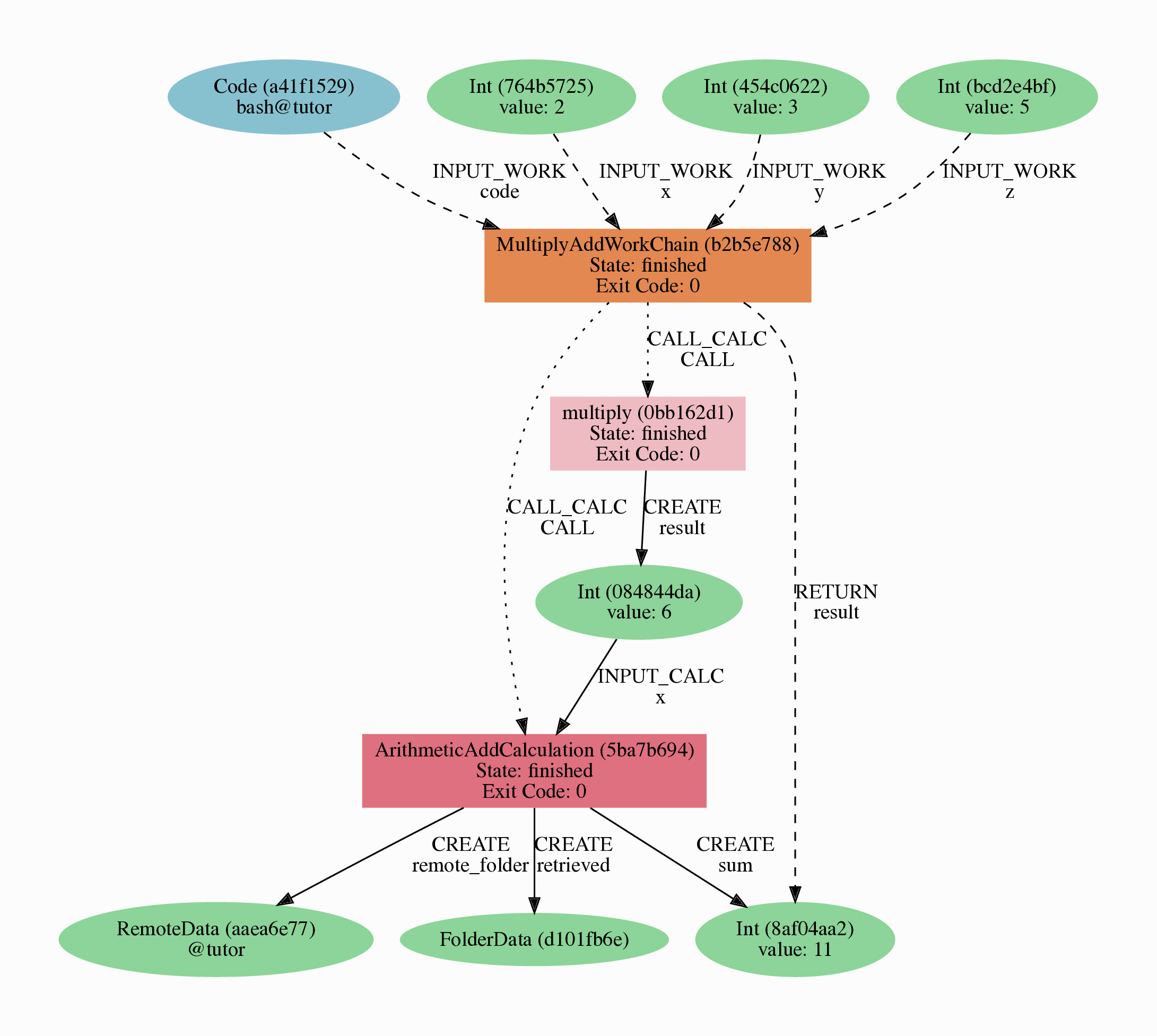
Fig. 2.1 Provenance Graph of a basic AiiDA WorkChain.¶

In the provenance graph, you can see different types of nodes represented by different shapes. The green ellipses are Data nodes, the blue ellipse is a Code node, and the rectangles represent processes, i.e. the calculations performed in your workflow.

The provenance graph allows us to not only see what data we have, but also how it was produced. During this basic tutorial we will first be using AiiDA to generate the provenance graph in Fig. 2.1, step by step.

2.2.2. Data nodes¶

Before running any calculations, let’s create and store a data node. AiiDA ships with an interactive IPython shell that has many basic AiiDA classes pre-loaded. To start the IPython shell, simply type in the terminal:

$ verdi shell

AiiDA implements data node types for the most common types of data (int, float, str, etc.), which you can extend with your own (composite) data node types if needed. For this tutorial, we’ll keep it very simple, and start by initializing an Int node and assigning it to the node variable:

In [1]: node = Int(2)

Note

Commands you have to execute in the bash terminal or the IPython shell can be clearly distinguished via the corresponding prompts and different box colors.

We can check the contents of the node variable like this:

In [2]: node
Out[2]: <Int: uuid: eac48d2b-ae20-438b-aeab-2d02b69eb6a8 (unstored) value: 2>

Quite a bit of information on our freshly created node is returned:

The data node is of the type Int
The node has the universally unique identifier (UUID) eac48d2b-ae20-438b-aeab-2d02b69eb6a8
The node is currently not stored in the database (unstored)
The integer value of the node is 2

Let’s store the node in the database:

In [3]: node.store()
Out[3]: <Int: uuid: eac48d2b-ae20-438b-aeab-2d02b69eb6a8 (pk: 1) value: 2>

As you can see, the data node has now been assigned a primary key (PK), a number that identifies the node in your database (pk: 1). The PK and UUID both reference the node with the only difference that the PK is unique for your local database only, whereas the UUID is a globally unique identifier and can therefore be used between different databases. Use the PK only if you are working within a single database, i.e. in an interactive session and the UUID in all other cases.

Important

The PK numbers shown throughout this first tutorial assume that you start from a completely empty database. It is possible that the nodes’ PKs will be different for your database!

The UUIDs are generated randomly and are therefore guaranteed to be different for nodes created during the tutorial.

Next, let’s leave the IPython shell by typing exit() and then enter. Back in the terminal, use the verdi command line interface (CLI) to check the data node we have just created:

$ verdi node show 1

This prints something like the following:

Property     Value
-----------  ------------------------------------
type         Int
pk           1
uuid         eac48d2b-ae20-438b-aeab-2d02b69eb6a8
label
description
ctime        2020-05-13 08:58:15.193421+00:00
mtime        2020-05-13 08:58:40.976821+00:00

Once again, we can see that the node is of type Int, has PK = 1, and UUID = eac48d2b-ae20-438b-aeab-2d02b69eb6a8. Besides this information, the verdi node show command also shows the (empty) label and description, as well as the time the node was created (ctime) and last modified (mtime).

Note

AiiDA already provides many standard data types, but you can also create your own.

2.2.3. Calculation functions¶

Once your data is stored in the database, it is ready to be used for some computational task. For example, let’s say you want to multiply two Int data nodes. The following Python function:

def multiply(x, y):
    return x * y

will give the desired result when applied to two Int nodes, but the calculation will not be stored in the provenance graph. However, we can use a Python decorator provided by AiiDA to automatically make it part of the provenance graph. Start up the AiiDA IPython shell again using verdi shell and execute the following code snippet:

In [1]: from aiida.engine import calcfunction
   ...:
   ...: @calcfunction
   ...: def multiply(x, y):
   ...:     return x * y

This converts the multiply function into an AiIDA calculation function, the most basic execution unit in AiiDA. Next, load the Int node you have created in the previous section using the load_node function and the PK of the data node:

In [2]: x = load_node(pk=1)

Of course, we need another integer to multiply with the first one. Let’s create a new Int data node and assign it to the variable y:

In [3]: y = Int(3)

Now it’s time to multiply the two numbers!

In [4]: multiply(x, y)
Out[4]: <Int: uuid: 42541d38-1fb3-4f60-8122-ab8b3e723c2e (pk: 4) value: 6>

Success! The calcfunction-decorated multiply function has multiplied the two Int data nodes and returned a new Int data node whose value is the product of the two input nodes. Note that by executing the multiply function, all input and output nodes are automatically stored in the database:

In [5]: y
Out[5]: <Int: uuid: 7865c8ff-f243-4443-9233-dd303a9be3c5 (pk: 2) value: 3>

We had not yet stored the data node assigned to the y variable, but by providing it as an input argument to the multiply function, it was automatically stored with PK = 2. Similarly, the returned Int node with value 6 has been stored with PK = 4.

Let’s once again leave the IPython shell with exit() and look for the process we have just run using the verdi CLI:

$ verdi process list

The returned list will be empty, but don’t worry! By default, verdi process list only returns the active processes. If you want to see all processes (i.e. also the processes that are terminated), simply add the -a option:

$ verdi process list -a

You should now see something like the following output:

  PK  Created    Process label    Process State    Process status
----  ---------  ---------------  ---------------  ----------------
   3  1m ago     multiply         ⏹ Finished [0]

Total results: 1

Info: last time an entry changed state: 1m ago (at 09:01:05 on 2020-05-13)

We can see that our multiply calcfunction was created 1 minute ago, assigned the PK 3, and has Finished.

As a final step, let’s have a look at the provenance of this simple calculation. The provenance graph can be automatically generated using the verdi CLI. Let’s generate the provenance graph for the multiply calculation function we have just run with PK = 3:

$ verdi node graph generate 3

Note

Remember that the PK of the calculation function can be different for your database.

The command will write the provenance graph to a .pdf file. You can open this file on the Amazon virtual machine by using evince:

$ evince 3.dot.pdf

If X-forwarding has been setup correctly, the provenance graph should appear on your local machine. In case the ssh connection is too slow, copy the file via scp to your local machine. To do so, if you are using Linux/Mac OS X, you can type in your local machine:

$ scp aiidatutorial:<path_to_the_graph_pdf> <local_folder>

and then open the file.

Note

You can also use the jupyter notebook setup explained here to download files. Note that while Firefox will display the PDF directly in the browser Chrome and Safari block viewing PDFs from jupyter notebook servers - with these browsers, you will need to tick the checkbox next to the PDF and download the file.

Alternatively, you can use graphical software to achieve the same, for instance: on Windows: WinSCP; on a Mac: Cyberduck; on Linux Ubuntu: using the ‘Connect to server’ option in the main menu after clicking on the desktop.

It should look something like the graph shown in Fig. 2.2.

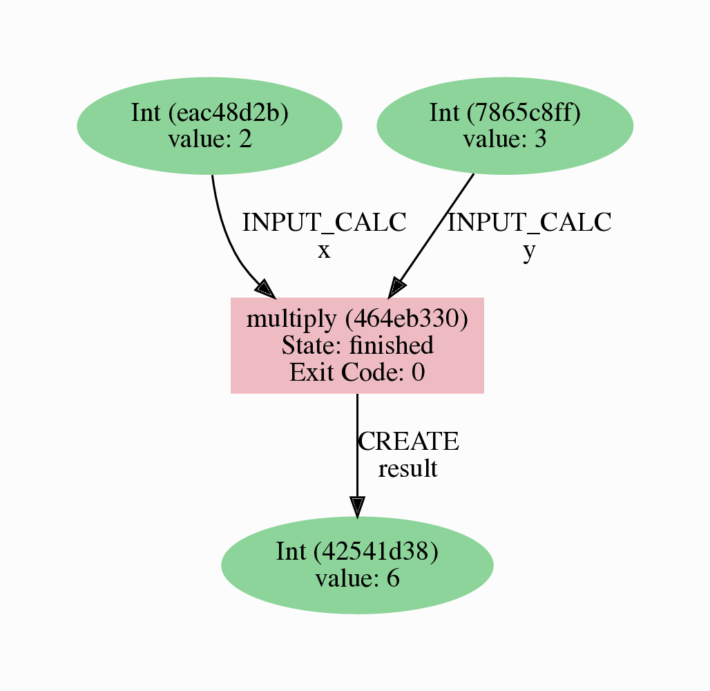
Fig. 2.2 Provenance graph of the multiply calculation function.¶

2.2.4. CalcJobs¶

When running calculations that require an external code or run on a remote machine, a simple calculation function is no longer sufficient. For this purpose, AiiDA provides the CalcJob process class. To run a CalcJob, you need to set up two things: a code that is going to implement the desired calculation and a computer for the calculation to run on. Let’s begin by setting up the computer using the verdi computer subcommand:

$ verdi computer setup -L tutor -H localhost -T local -S direct -w `echo $PWD/work` -n
$ verdi computer configure local tutor --safe-interval 5 -n

The first commands sets up the computer with the following options:

label (-L): tutor
hostname (-H): localhost
transport (-T): local
scheduler (-S): direct
work-dir (-w): The work subdirectory of the current directory

The second command configures the computer with a minimum interval between connections (--safe-interval) of 5 seconds. For both commands, the non-interactive option (-n) is added to not prompt for extra input.

Next, let’s set up the code we’re going to use for the tutorial:

$ verdi code setup -L add --on-computer --computer=tutor -P arithmetic.add --remote-abs-path=/bin/bash -n

This command sets up a code with label add on the computer tutor, using the plugin arithmetic.add.

A typical real-world example of a computer is a remote supercomputing facility. Codes can be anything from a Python script to powerful ab initio codes such as Quantum ESPRESSO or machine learning tools like Tensorflow. Let’s have a look at the codes that are available to us:

$ verdi code list
# List of configured codes:
# (use 'verdi code show CODEID' to see the details)
* pk 5 - add@tutor

You can see a single code add@tutor, with PK = 5, in the printed list. This code allows us to add two integers together. The add@tutor identifier indicates that the code with label add is run on the computer with label tutor. To see more details about the computer, you can use the following verdi command:

$ verdi computer show tutor
Computer name:     tutor
 * PK:             1
 * UUID:           b9ecb07c-d084-41d7-b862-a2b1f02722c5
 * Description:
 * Hostname:       localhost
 * Transport type: local
 * Scheduler type: direct
 * Work directory: /Users/mbercx/epfl/tutorials/my_tutor/work
 * Shebang:        #!/bin/bash
 * mpirun command: mpirun -np {tot_num_mpiprocs}
 * prepend text:
 # No prepend text.
 * append text:
 # No append text.

We can see that the Work directory has been set up as the work subdirectory of the current directory. This is the directory in which the calculations running on the tutor computer will be executed.

Note

You may have noticed that the PK of the tutor computer is 1, same as the Int node we created at the start of this tutorial. This is because different entities, such as nodes, computers and groups, are stored in different tables of the database. So, the PKs for each entity type are unique for each database, but entities of different types can have the same PK within one database.

Let’s now start up the verdi shell again and load the add@tutor code using its label:

In [1]: code = load_code(label='add')

Every code has a convenient tool for setting up the required input, called the builder. It can be obtained by using the get_builder method:

In [2]: builder = code.get_builder()

Using the builder, you can easily set up the calculation by directly providing the input arguments. Let’s use the Int node that was created by our previous calcfunction as one of the inputs and a new node as the second input:

In [3]: builder.x = load_node(pk=4)
   ...: builder.y = Int(5)

In case that your nodes’ PKs are different and you don’t remember the PK of the output node from the previous calculation, check the provenance graph you generated earlier and use the UUID of the output node instead:

In [3]: builder.x = load_node(uuid='42541d38')
   ...: builder.y = Int(5)

Note that you don’t have to provide the entire UUID to load the node. As long as the first part of the UUID is unique within your database, AiiDA will find the node you are looking for.

Note

One nifty feature of the builder is the ability to use tab completion for the inputs. Try it out by typing builder. + <TAB> in the verdi shell.

To execute the CalcJob, we use the run function provided by the AiiDA engine:

In [4]: from aiida.engine import run
   ...: run(builder)

Wait for the process to complete. Once it is done, it will return a dictionary with the output nodes:

Out[4]:
{'sum': <Int: uuid: 7d5d781e-8f17-498a-b3d5-dbbd3488b935 (pk: 8) value: 11>,
'remote_folder': <RemoteData: uuid: 888d654a-65fb-4da0-b3bc-d63f0374f274 (pk: 9)>,
'retrieved': <FolderData: uuid: 4733aa78-2e2f-4aeb-8e09-c5cfb58553db (pk: 10s)>}

Besides the sum of the two Int nodes, the calculation function also returns two other outputs: one of type RemoteData and one of type FolderData. See the topics section on calculation jobs for more details. Now, exit the IPython shell and once more check for all processes:

$ verdi process list -a

You should now see two processes in the list. One is the multiply calcfunction you ran earlier, the second is the ArithmeticAddCalculation CalcJob that you have just run. Grab the PK of the ArithmeticAddCalculation, and generate the provenance graph. The result should look like the graph shown in Fig. 2.3.

$ verdi node graph generate 7

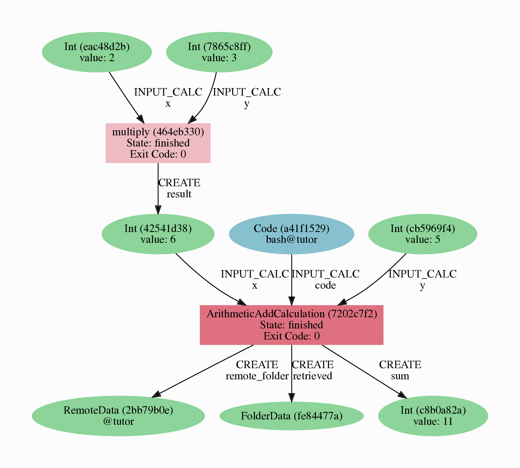
Fig. 2.3 Provenance graph of the ArithmeticAddCalculation CalcJob, with one input provided by the output of the multiply calculation function.¶

You can see more details on any process, including its inputs and outputs, using the verdi shell:

$ verdi process show 7

2.2.5. Submitting to the daemon¶

When we used the run command in the previous section, the IPython shell was blocked while it was waiting for the CalcJob to finish. This is not a problem when we’re simply multiplying two numbers, but if we want to run multiple calculations that take hours or days, this is no longer practical. Instead, we are going to submit the CalcJob to the AiiDA daemon. The daemon is a program that runs in the background and manages submitted calculations until they are terminated. Let’s first check the status of the daemon using the verdi CLI:

$ verdi daemon status

If the daemon is running, the output will be something like the following:

Profile: tutorial
Daemon is running as PID 96447 since 2020-05-22 18:04:39
Active workers [1]:
  PID    MEM %    CPU %  started
-----  -------  -------  -------------------
96448    0.507        0  2020-05-22 18:04:39
Use verdi daemon [incr | decr] [num] to increase / decrease the amount of workers

In this case, let’s stop it for now:

$ verdi daemon stop

Next, let’s submit the CalcJob we ran previously. Start the verdi shell and execute the Python code snippet below. This follows all the steps we did previously, but now uses the submit function instead of run:

In [1]: from aiida.engine import submit
   ...:
   ...: code = load_code(label='add')
   ...: builder = code.get_builder()
   ...: builder.x = load_node(pk=4)
   ...: builder.y = Int(5)
   ...:
   ...: submit(builder)

When using submit the calculation job is not run in the local interpreter but is sent off to the daemon and you get back control instantly. Instead of the result of the calculation, it returns the node of the CalcJob that was just submitted:

Out[1]: <CalcJobNode: uuid: e221cf69-5027-4bb4-a3c9-e649b435393b (pk: 12) (aiida.calculations:arithmetic.add)>

Let’s exit the IPython shell and have a look at the process list:

$ verdi process list

You should see the CalcJob you have just submitted, with the state Created:

  PK  Created    Process label             Process State    Process status
----  ---------  ------------------------  ---------------  ----------------
  12  13s ago    ArithmeticAddCalculation  ⏹ Created

Total results: 1

Info: last time an entry changed state: 13s ago (at 09:06:57 on 2020-05-13)

The CalcJob process is now waiting to be picked up by a daemon runner, but the daemon is currently disabled. Let’s start it up (again):

$ verdi daemon start

Now you can either use verdi process list to follow the execution of the CalcJob, or watch its progress:

$ verdi process watch 12

Let’s wait for the CalcJob to complete (state changes to “finished”). Quit the watch command (Ctrl+C) and use verdi process list -a to see all processes we have run so far:

  PK  Created    Process label             Process State    Process status
----  ---------  ------------------------  ---------------  ----------------
   3  6m ago     multiply                  ⏹ Finished [0]
   7  2m ago     ArithmeticAddCalculation  ⏹ Finished [0]
  12  1m ago     ArithmeticAddCalculation  ⏹ Finished [0]

Total results: 3

Info: last time an entry changed state: 14s ago (at 09:07:45 on 2020-05-13)

2.2.6. Workflows¶

So far we have executed each process manually. AiiDA allows us to automate these steps by linking them together in a workflow, whose provenance is stored to ensure reproducibility. For this tutorial we have prepared a basic WorkChain that is already implemented in aiida-core. You will see the details of this code in the section on basic workflows.

Note

Besides WorkChain’s, workflows can also be implemented as work functions. These are ideal for workflows that are not very computationally intensive and can be easily implemented in a Python function.

Let’s run the WorkChain above! Start up the verdi shell and load the MultiplyAddWorkChain using the WorkflowFactory:

In [1]: MultiplyAddWorkChain = WorkflowFactory('arithmetic.multiply_add')

The WorkflowFactory is a useful and robust tool for loading workflows based on their entry point, e.g. 'arithmetic.multiply_add' in this case. Similar to a CalcJob, the WorkChain input can be set up using a builder:

In [2]: builder = MultiplyAddWorkChain.get_builder()
   ...: builder.code = load_code(label='add')
   ...: builder.x = Int(2)
   ...: builder.y = Int(3)
   ...: builder.z = Int(5)

Once the WorkChain input has been set up, we submit it to the daemon using the submit function from the AiiDA engine:

In [3]: from aiida.engine import submit
   ...: submit(builder)

Now quickly leave the IPython shell and check the process list:

$ verdi process list -a

Depending on which step the workflow is running, you should get something like the following:

  PK  Created    Process label             Process State    Process status
----  ---------  ------------------------  ---------------  ------------------------------------
   3  7m ago     multiply                  ⏹ Finished [0]
   7  3m ago     ArithmeticAddCalculation  ⏹ Finished [0]
  12  2m ago     ArithmeticAddCalculation  ⏹ Finished [0]
  19  16s ago    MultiplyAddWorkChain      ⏵ Waiting        Waiting for child processes: 22
  20  16s ago    multiply                  ⏹ Finished [0]
  22  15s ago    ArithmeticAddCalculation  ⏵ Waiting        Waiting for transport task: retrieve

Total results: 6

Info: last time an entry changed state: 0s ago (at 09:08:59 on 2020-05-13)

We can see that the MultiplyAddWorkChain is currently waiting for its child process, the ArithmeticAddCalculation, to finish. Check the process list again for all processes (You should know how by now!). After about half a minute, all the processes should be in the Finished state.

We can now generate the full provenance graph for the WorkChain with:

$ verdi node graph generate 19

Open the generated pdf file using evince. Look familiar? The provenance graph should be similar to the one we showed at the start of this tutorial (Fig. 2.4).

Fig. 2.4 Final provenance Graph of the basic AiiDA tutorial.¶

2.3. Real world example using Quantum ESPRESSO¶

So far we’ve covered the AiiDA basics using data nodes and processes involving simple arithmetic. In the second part of this session, we’ll have a look at some more interesting data structures and calculations, based on some examples using Quantum ESPRESSO.

2.3.1. Importing data¶

Before we start running Quantum ESPRESSO calculations ourselves, which is the topic of the next session, we are going to look at an AiiDA database already created by someone else. Let’s import one from the web:

$ verdi import https://object.cscs.ch/v1/AUTH_b1d80408b3d340db9f03d373bbde5c1e/marvel-vms/tutorials/aiida_tutorial_2020_07_perovskites_v0.9.aiida

As mentioned previously, AiiDA databases contain not only results of calculations but also their inputs and information on how a particular result was obtained. This information, the data provenance, is stored in the form of a directed acyclic graph (DAG). In the following, we are going to introduce you to different ways of browsing this graph and will ask you to find out some information regarding the database you just imported.

2.3.2. The provenance graph¶

Fig. 2.5 shows a typical example of a Quantum ESPRESSO calculation represented in an AiiDA graph. Have a look to the figure and its caption before moving on.

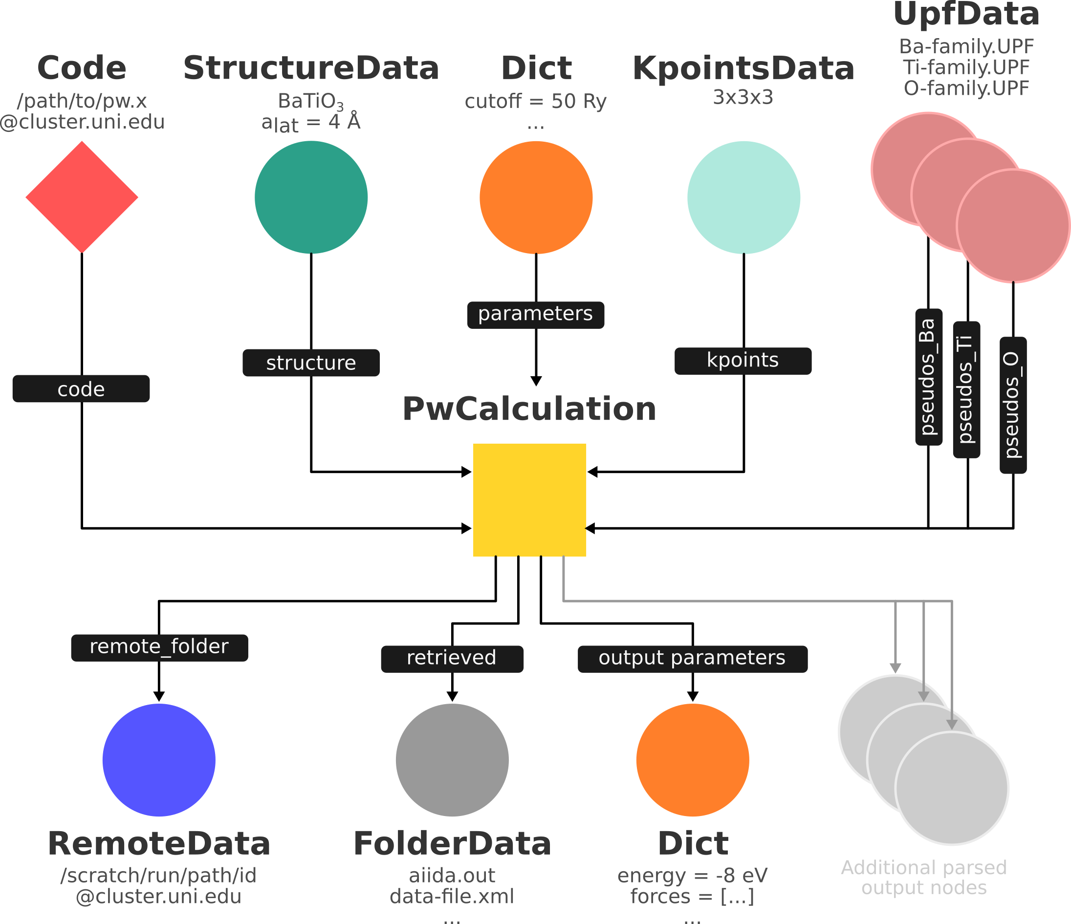
Fig. 2.5 Graph with all inputs (data, circles; and code, diamond) to the Quantum ESPRESSO calculation (square) that you will create in the Running computations section of this tutorial. Besides the inputs, the graph also shows the outputs that the engine will create and connect automatically. The RemoteData node is created during submission and can be thought as a symbolic link to the remote folder in which the calculation runs on the cluster. The other nodes are created when the calculation has finished, after retrieval and parsing. The node with linkname retrieved contains the relevant raw output files stored in the AiiDA repository; all other nodes are added by the parser. Additional nodes (symbolized in gray) can be added by the parser: e.g., an output StructureData if you performed a relaxation calculation, a TrajectoryData for molecular dynamics, etc.¶

Fig. 2.5 was drawn by hand but you can generate a similar graph automatically by passing the identifier of a calculation node to verdi node graph generate <IDENTIFIER>, or using the graph’s python API. Remember that identifiers in AiiDA can come in several forms:

“Primary Key” (PK): An integer, e.g. 723, that identifies your entity within your database (automatically assigned)

Universally Unique Identifier (UUID): A string, e.g. ce81c420-7751-48f6-af8e-eb7c6a30cec3 that identifies your entity globally (automatically assigned)

Label: A human-readable string, e.g. test_qe_calculation (manually assigned)

Any verdi command that expects an identifier will accept a PK, a UUID or a label (although not all entities have a label by default). While PKs are often shorter than UUIDs and can be easier to remember, they are only unique within your database. Whenever you intend to share your data with others, use UUIDs to refer to nodes.

Note

For UUIDs, it is sufficient to specify a subset (starting at the beginning) as long as it can already be uniquely resolved. For more information on identifiers in verdi and AiiDA in general, see the documentation.

Let’s generate a graph for the calculation node with UUID ce81c420-7751-48f6-af8e-eb7c6a30cec3:

$ verdi node graph generate ce81c420

This command will create the file <PK>.dot.pdf that can be viewed with any PDF document viewer. See the notes on how to open the pdf on AWS in case you need a quick reminder on how to do so.

For the remainder of this section, we’ll use the verdi CLI and the verdi shell to explore the properties of the PwCalculation, as well as its inputs. Understanding these data types will come in handy for the section on running calculations. We’ll also introduce some new CLI commands and shell features that will be useful for the hands-on sessions that follow.

2.3.3. Processes¶

Anything that ‘runs’ in AiiDA, be it calculations or workflows, is considered a Process. Let’s have another look at the finished processes in the database by passing the -S/--process-state flag:

$ verdi process list -S finished

This command will list all the processes that have a process state Finished and should contain a list of PwCalculation processes that you have just imported:

PK    Created    Process label   Process State    Process status
----  ---------  --------------  ---------------  ----------------
...
1178  1653D ago  PwCalculaton    ⏹ Finished [0]
1953  1653D ago  PwCalculaton    ⏹ Finished [0]
1734  1653D ago  PwCalculaton    ⏹ Finished [0]
 336  1653D ago  PwCalculaton    ⏹ Finished [0]
1056  1653D ago  PwCalculaton    ⏹ Finished [0]
1369  1653D ago  PwCalculaton    ⏹ Finished [0]
...

Total results: 177

Info: last time an entry changed state: 21m ago (at 20:03:00 on 2020-07-03)

Note that processes can be in any of the following states:

Created

Waiting

Running

Finished

Excepted

Killed

The first three states are ‘active’ states, meaning the process is not done yet, and the last three are ‘terminal’ states. Once a process is in a terminal state, it will never become active again. The official documentation contains more details on process states.

Remember that in order to list processes of all states, you can use the -a/--all flag:

$ verdi process list -a

This command will list all the processes that have ever been launched. As your database will grow, so will the output of this command. To limit the number of results, you can use the -p/--past-days <NUM> option, that will only show processes that were created NUM days ago. For example, this lists all processes launched since yesterday:

$ verdi process list -a -p1

This will be useful in the coming days to limit the output from verdi process list. Each row of the output identifies a process with some basic information about its status. For a more detailed list of properties, you can use verdi process show, but to address any specific process, you need an identifier for it.

Let’s revisit the process with the UUID ce81c420-7751-48f6-af8e-eb7c6a30cec3, this time using the CLI:

$ verdi process show ce81c420

Producing the output:

Property     Value
-----------  ------------------------------------
type         PwCalculation
state        Finished [0]
pk           630
uuid         ce81c420-7751-48f6-af8e-eb7c6a30cec3
label
description
ctime        2014-10-27 17:51:21.781045+00:00
mtime        2019-05-09 14:10:09.307986+00:00
computer     [1] daint

Inputs      PK    Type
----------  ----  -------------
pseudos
    Ba      1092  UpfData
    O       1488  UpfData
    Ti      1855  UpfData
code        631   Code
kpoints     498   KpointsData
parameters  629   Dict
settings    500   Dict
structure   1133  StructureData

Outputs                    PK  Type
-----------------------  ----  -------------
output_kpoints           1455  KpointsData
output_parameters         789  Dict
output_structure          788  StructureData
output_trajectory_array   790  ArrayData
remote_folder            1811  RemoteData
retrieved                 787  FolderData

Compare the in- and outputs with those visualized in the provenance graph earlier. The PKs shown for the inputs and outputs will come in handy to get more information about those nodes, which we’ll do for several inputs below.

You can also use the verdi CLI to obtain the content of the raw input file to Quantum ESPRESSO (that was generated by AiiDA) via the command:

$ verdi calcjob inputcat ce81c420

where you once again provide the identifier of the PwCalculation process, which is a calculation job (hence the calcjob subcommand). This will print the input file of the Quantum ESPRESSO calculation, which when run through AiiDA is written to the default input file aiida.in. To see a list of all the files used to run a calculation (input file, submission script, etc.) instead type:

$ verdi calcjob inputls ce81c420

Adding the --color flag helps distinguishing files from folders. Once you know the name of the file you want to visualize, you can call the verdi calcjob inputcat [PATH] command specifying the path of the file to show. For instance, to see the submission script, you can use:

$ verdi calcjob inputcat ce81c420 _aiidasubmit.sh

2.3.4. Inputs¶

Here we will discuss the input nodes of the PwCalculation calculation job. The Code node and its setup will be discussed in the next hands-on on running computations.

2.3.4.1. Dict - parameters¶

Let’s investigate some of the input and output nodes of the PwCalculation. Dictionaries with various parameters are represented in AiiDA by Dict nodes. From the inputs of the process, let’s choose the node of type Dict with input link name parameters and type in the terminal:

$ verdi data dict show <IDENTIFIER>

where <IDENTIFIER> is the PK of the node.

A Dict node contains a dictionary (i.e. key–value pairs), stored in the database in a format ready to be queried. We will learn how to run queries during the hands-on session on working with data and querying your results. The command above will print the content dictionary, containing the parameters used to define the input file for the calculation.

Check the consistency of the parameters stored in the Dict node with those written in the aiida.in input file you printed previously. Even if you don’t know the meaning of the input flags of a Quantum ESPRESSO calculation, you should be able to see how the input dictionary has been converted to Fortran namelists.

Of course, we can also load the contents of the parameters dictionary in Python. Start up a verdi shell and load the Dict node:

In [1]: params = load_node(PK)

Next, we can use the get_dict() method to obtain the dictionary stored in the Dict node:

In [2]: pw_dict = params.get_dict()

In [3]: pw_dict
Out[3]:
{'SYSTEM': {'nspin': 2,
  'degauss': 0.02,
  'ecutrho': 600,
  'ecutwfc': 60,
  'smearing': 'gaussian',
  'occupations': 'smearing',
  'starting_magnetization': [0.5, 0.5, 0.1]},
 'CONTROL': {'wf_collect': True,
  'calculation': 'vc-relax',
  'max_seconds': 1710,
  'restart_mode': 'from_scratch'},
 'ELECTRONS': {'conv_thr': 1e-10,
  'mixing_beta': 0.7,
  'mixing_mode': 'plain',
  'diagonalization': 'david',
  'electron_maxstep': 50}}

Modify the python dictionary pw_dict so that the wave-function cutoff is now set to 20 Ry. Objects that are already stored in the database cannot be modified, as doing so would alter the provenance graph of connected nodes. So, to write the modified dictionary to the database, you have to create a new object of class Dict. To load any data class, we can use AiiDA’s DataFactory and the entry point of the Dict class ('dict'):

In [4]: Dict = DataFactory('dict')
   ...: new_params = Dict(dict=pw_dict)

where pw_dict is the modified python dictionary. Note that at this point new_params is not yet stored in the database. Let’s finish this example by storing the new_params dictionary node in the database:

In [5]: new_params.store()

Note

While it is also possible to import the Dict class directly, it is recommended to use the DataFactory function instead, as this is more future-proof: even if the import path of the class changes in the future, its entry point string ('dict') will remain stable.

2.3.4.2. StructureData¶

Next, let’s have a look at the StructureData node, which represents a crystalline structure. We can consider for instance the input structure to the calculation we were considering before (it should have the UUID 3a4b1270). Such objects can be inspected interactively by means of an atomic viewer such as the one provided by ase. AiiDA however supports several other viewers such as xcrysden, jmol, and vmd. Type in the terminal:

$ verdi data structure show --format ase <IDENTIFIER>

to show the selected structure, although it will take a few seconds to appear (it has to go over a tunnel on your SSH connection). You should be able to rotate the view with the right mouse button.

Note

If you receive some errors, make sure your X-forwarding settings have been set up correctly, as explained in the setup section.

Alternatively, especially if showing them interactively is too slow over SSH, you can export the content of a structure node in various popular formats such as xyz, xsf or cif. This is achieved by typing in the terminal:

$ verdi data structure export --format xsf <IDENTIFIER> > BaTiO3.xsf

This outputs the structure in xsf format and writes it to a file.

You can open the generated xsf file and observe the cell and the coordinates. Then, you can then copy BaTiO3.xsf from the Amazon machine to your local one and then visualize it, e.g. with xcrysden (if you have it installed):

$ xcrysden --xsf BaTiO3.xsf

The StructureData node can also be investigated using the verdi shell. First, open the verdi shell and load the structure node:

In [1]: structure = load_node('3a4b1270')
In [2]: structure
Out[2]: <StructureData: uuid: 3a4b1270-82bf-4d66-a51f-982294f6e1b3 (pk: 1161)>

You can display its chemical formula using:

In [3]: structure.get_formula()
Out[3]: 'BaO3Ti'

or, to obtain the atomic positions and species:

In [4]: structure.sites
Out[4]:
[<Site: kind name 'Ba' @ 0.0,1.78886419607596e-30,0.0>,
 <Site: kind name 'Ti' @ 1.98952035955311,1.98952035955311,1.98952035955311>,
 <Site: kind name 'O' @ 1.98952035955311,1.98952035955311,0.0>,
 <Site: kind name 'O' @ 1.98952035955311,2.33671938655715e-31,1.98952035955311>,
 <Site: kind name 'O' @ 0.0,1.98952035955311,1.98952035955311>]

If you are familiar with ASE and Pymatgen, you can convert this structure to those formats by typing either

In [5]: structure.get_ase()
Out[5]: Atoms(symbols='BaTiO3', pbc=True, cell=[3.97904071910623, 3.97904071910623, 3.97904071910623], masses=...)

In [6]: structure.get_pymatgen()
Out[6]:
Structure Summary
Lattice
    abc : 3.97904071910623 3.97904071910623 3.97904071910623
 angles : 90.0 90.0 90.0
 volume : 62.999216807333035
      A : 3.97904071910623 0.0 0.0
      B : 0.0 3.97904071910623 0.0
      C : 0.0 0.0 3.97904071910623
PeriodicSite: Ba (0.0000, 0.0000, 0.0000) [0.0000, 0.0000, 0.0000]
PeriodicSite: Ti (1.9895, 1.9895, 1.9895) [0.5000, 0.5000, 0.5000]
PeriodicSite: O (1.9895, 1.9895, 0.0000) [0.5000, 0.5000, 0.0000]
PeriodicSite: O (1.9895, 0.0000, 1.9895) [0.5000, 0.0000, 0.5000]
PeriodicSite: O (0.0000, 1.9895, 1.9895) [0.0000, 0.5000, 0.5000]

Of course, the structure above is already in our database, after we imported it at the start of this section. In order to add new structures to your AiiDA database, you can also define a structure by hand, or import it from an online repository:

2.3.4.3. KpointsData¶

A set of k-points in the Brillouin zone is represented by an instance of the KpointsData class. Look for an identifier (PK or UUID) of the KpointsData input node of the PwCalculation whose provenance graph you generated earlier, and load the node in the verdi shell:

In [1]: kpoints = load_node(<IDENTIFIER>)

You can get the k-points mesh using:

In [2]: kpoints.get_kpoints_mesh()
Out[2]: ([6, 6, 6], [0.0, 0.0, 0.0])

To get the full (explicit) list of k-points belonging to this mesh, use:

In [3]: kpoints.get_kpoints_mesh(print_list=True)
Out[3]:
array([[0.        , 0.        , 0.        ],
       [0.        , 0.        , 0.16666667],
       ...
       [0.83333333, 0.83333333, 0.66666667],
       [0.83333333, 0.83333333, 0.83333333]])

If this throws an AttributeError, it means that the kpoints instance does not represent a regular mesh but rather a list of k-points defined by their crystal coordinates (typically used when plotting a band structure). In this case, get the list of k-points coordinates using

In [3]: kpoints.get_kpoints()

Conversely, if the KpointsData node does actually represent a mesh, this method is the one, that when called, will throw an AttributeError.

If you prefer Cartesian (rather than fractional) coordinates, type:

In [4]: kpoints.get_kpoints(cartesian=True)

For later use in this tutorial, let us try now to create a k-points instance, to describe a regular (2 x 2 x 2) mesh of k-points, centered at the Gamma point (i.e. without offset). This can be done with the following set of commands:

In [5]: KpointsData = DataFactory('array.kpoints')
   ...: kpoints = KpointsData()
   ...: kpoints.set_kpoints_mesh([2, 2, 2])

Here, we first load the KpointsData class using the DataFactory and the entry point (array.kpoints). Then, we create an instance of the KpointData class, and use the set_kpoints_mesh() method to set the mesh to a regular 2x2x2 Gamma-point centered mesh.

2.3.4.4. Pseudopotentials¶

From the graph you generated in section The provenance graph, find the UUID of the pseudopotential file (LDA). Load it and show what elements it corresponds to by typing:

In [1]: upf = load_node('<UUID>')
   ...: upf.element

All methods of UpfData are accessible by typing upf. and then pressing TAB.

Pseudopotentials in AiiDA are grouped in ‘families’ that contain one single pseudo per element. We will see how to work with UPF pseudopotentials (the format used by Quantum ESPRESSO and some other codes). Download and untar the SSSP pseudopotentials via the commands:

$ mkdir sssp_pseudos
$ wget 'https://archive.materialscloud.org/record/file?filename=SSSP_1.1_PBE_efficiency.tar.gz&record_id=23&file_id=d2ce4186-bf76-4e05-8b39-444b4da30273' -O SSSP_1.1_PBE_efficiency.tar.gz
$ tar -C sssp_pseudos -zxvf SSSP_1.1_PBE_efficiency.tar.gz

Then you can upload the whole set of pseudopotentials to AiiDA by using the following verdi command:

$ verdi data upf uploadfamily sssp_pseudos 'SSSP' 'SSSP pseudopotential library'

In the command above, sssp_pseudos is the folder containing the pseudopotentials, 'SSSP' is the label given to the family, and the last argument is its description. Finally, you can list all the pseudo families present in the database with

$ verdi data upf listfamilies

2.3.4.5. (Optional section) Comments¶

AiiDA offers the possibility to attach comments to a any node, in order to be able to remember more easily its details. Node with UUID prefix ce81c420 should have no comments, but you can add a very instructive one by typing in the terminal:

$ verdi node comment add "vc-relax of a BaTiO3 done with QE pw.x" -N <IDENTIFIER>

Now, if you ask for a list of all comments associated to that calculation by typing:

$ verdi node comment show <IDENTIFIER>

the comment that you just added will appear together with some useful information such as its creator and creation date. We let you play with the other options of verdi node comment command to learn how to update or remove comments.

Footnotes

1: We purposefully do not provide advanced commands for crystal structure manipulation in AiiDA, because python packages that accomplish such tasks already exist (such as ASE or pymatgen).