6. A real-world WorkChain: Computing a band structure
As a final demonstration of the power of WorkChains in AiiDA, we want to give a demonstration of a WorkChain, which will take a structure as its only input and compute its band structure.
All of the steps that would normally have to be done manually by the researcher – choosing appropriate pseudopotentials, energy cutoffs, k-point meshes, high-symmetry k-point paths, and performing the various calculation steps – are performed automatically by the WorkChain.
The demonstration of the WorkChain will be performed in a Jupyter notebook, that you can download from here (or you can find a rendered vesion below, at the end of this page).
There you will find some example structures that are loaded from the Crystallography Open Database (COD), using the COD-importer integrated in AiiDA.
Note that the required time to calculate the bandstructure for the given structures ranges from ~5 minutes to more than an hour, given that the virtual machine is running on two cores with CPU throttling. It is not necessary to run all these examples as they may take too long to complete. For reference, the expected output band structures are plotted in Fig. 6.1 to Fig. 6.4.
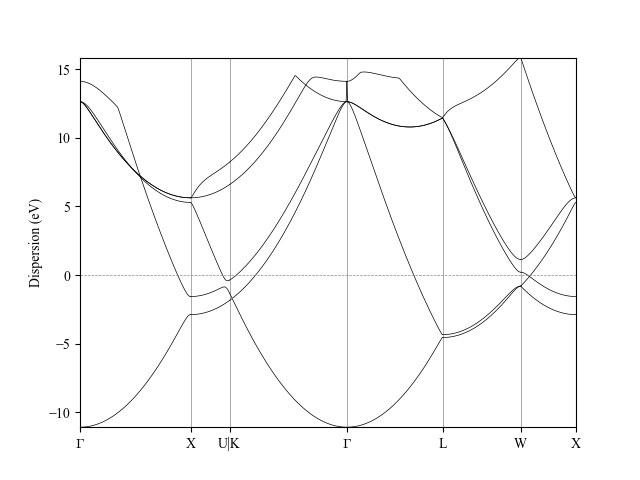
Fig. 6.1 Electronic band structures of Al computed with AiiDA’s PwBandsWorkChain
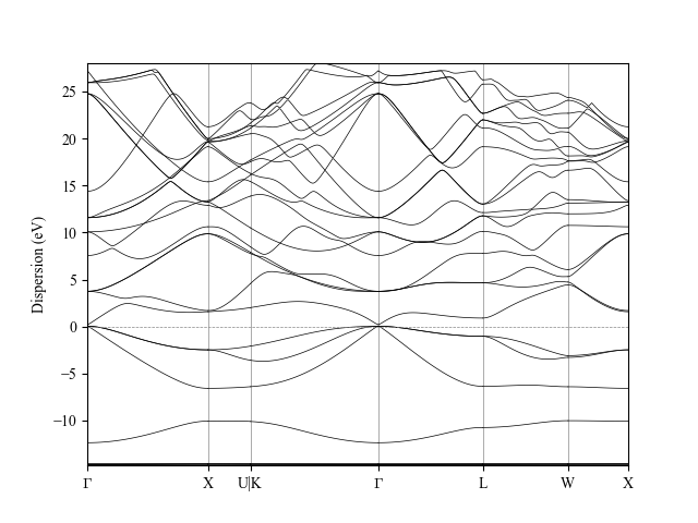
Fig. 6.2 Electronic band structures of GaAs computed with AiiDA’s PwBandsWorkChain
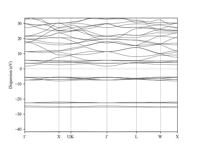
Fig. 6.3 Electronic band structures of CaF2 computed with AiiDA’s PwBandsWorkChain
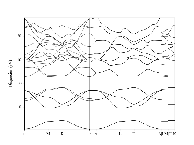
Fig. 6.4 Electronic band structures of BN computed with AiiDA’s PwBandsWorkChain