1. Quantum ESPRESSO

We’ll start with a quick demo of how AiiDA can make your life easier as a computational scientist.

Note

Throughout this tutorial we will be using the verdi command line interface (CLI). Here’s couple of tricks that will make your life easier:

• The verdi command supports tab-completion: In the terminal, type verdi, followed by a space and press the ‘Tab’ key twice to show a list of all the available sub commands.

• For help on verdi or any of its subcommands, simply append the --help/-h flag:

  $ verdi -h
  

1.1. Importing a structure and inspecting it

First, download the Si structure file: Si.cif. You can download the file easily using wget:

$ wget https://aiida-tutorials.readthedocs.io/en/tutorial-2021-abc/_downloads/1383def58ffe702e2911585fea20e33d/Si.cif

Note

You may have noticed that on the top right of each code block there a button for copying the contents of the block. This nifty feature will only copy the commands that needs to be executed, but note that in some code snippets you might still have to replace some of the content! On the AiiDAlab cluster you will be able to use the usual short-key of your operating system to paste the contents (Ctrl+V or Command+V), but in the terminal of the Quantum Mobile machine you will need to add Shift (Shift+Ctrl+V).

Next, you can import it into your database with the verdi CLI.

$ verdi data structure import ase Si.cif
  Successfully imported structure Si2 (PK = 1)

Each piece of data in AiiDA gets a PK number (a “primary key”) that identifies it in your database. This is printed out on the screen by the verdi data structure import command. It’s a good idea to mark it down, but should you forget, you can always have a look at the structures in the database using:

$ verdi data structure list
  Id  Label    Formula
----  -------  ---------
   1           Si2

The first column (marked Id) are the PK’s of the StructureData nodes.

Important

If you are starting this tutorial with an empty database, as in this example, the Si structure node PK will also be 1. If not, the PK numbers shown throughout this tutorial will be different for your database! Throughout this section, replace the string <PK> with the appropriate PK number.

Let us first inspect the node you just created:

$ verdi node show <PK>
Property     Value
-----------  ------------------------------------
type         StructureData
pk           1
uuid         ddb8c21c-2d3f-4374-aa86-44f8bb84aa3f
label
description
ctime        2021-02-09 20:57:03.304174+00:00
mtime        2021-02-09 20:57:03.421210+00:00

You can see some information on the node, including its type (StructureData, the AiiDA data type for storing crystal structures), a label and a description (empty for now, can be changed), a creation time (ctime) and a last modification time (mtime), the PK of the node and its UUID (universally unique identifier). The PK and UUID both reference the node with the only difference that the PK is unique for your local database only, whereas the UUID is a globally unique identifier and can therefore be used between different databases.

Important

The UUIDs are generated randomly and are therefore guaranteed to be different from the ones shown here. In the commands that follow, remember to replace <PK>, or <UUID> by the appropriate identifier.

1.2. Running a calculation

We’ll start with running a simple self-consistent field calculation (SCF) with Quantum ESPRESSO for the structure we just imported. First, we’ll need to make sure we have set up the Quantum ESPRESSO code in our database. This will depend on whether you are running the tutorial in the Quantum Mobile or the AiiDAlab cluster:

Quantum MobileAiiDAlab cluster

Let’s have a look at the codes in our database with the verdi shell:

$ verdi code list
# List of configured codes:
# (use 'verdi code show CODEID' to see the details)
* pk 1 - qe-3.4.0-pw@localhost
* pk 2 - qe-3.4.0-cp@localhost
* pk 3 - qe-3.4.0-pp@localhost
* pk 4 - qe-3.4.0-ph@localhost
* pk 5 - qe-3.4.0-neb@localhost
* pk 6 - qe-3.4.0-projwfc@localhost
* pk 7 - qe-3.4.0-pw2wannier90@localhost
* pk 8 - qe-3.4.0-q2r@localhost
* pk 9 - qe-3.4.0-dos@localhost
* pk 10 - qe-3.4.0-matdyn@localhost

As you can see, this Quantum Mobile virtual machine already comes with all of the Quantum ESPRESSO codes set up in the AiiDA database. The code we will be running is the pw.x code, set up under the label qe-3.4.0-pw on the localhost computer. Make a note of the PK or label of the code, since you’ll need to replace it in code snippets later in this tutorial.

To run the SCF calculation, we’ll also need to provide the family of pseudopotentials. These can be installed easily using the aiida-pseudo package:

$ aiida-pseudo install sssp
Info: downloading selected pseudo potentials archive...  [OK]
Info: downloading selected pseudo potentials metadata...  [OK]
Info: unpacking archive and parsing pseudos...  [OK]
Success: installed `SSSP/1.1/PBE/efficiency` containing 85 pseudo potentials

This command will install the SSSP library version 1.1. To see if the pseudopotential families have been installed correctly, do:

$ aiida-pseudo list
Label                    Type string         Count
-----------------------  ------------------  -------
SSSP/1.1/PBE/efficiency  pseudo.family.sssp  85

Along with the PK of the StructureData node for the silicon structure that we imported in the previous section, we now have everything to set up the calculation step by step. Before doing so we will first shut down the AiiDA daemon. The daemon is a program that runs in the background and manages submitted calculations until they are terminated. Check the status of the daemon using the verdi CLI:

$ verdi daemon status

If the daemon is running, the output will be something like the following:

Profile: default
Daemon is running as PID 1033 since 2020-11-29 14:37:59
Active workers [1]:
PID    MEM %    CPU %  started
-----  -------  -------  -------------------
1036    0.415        0  2020-11-29 14:38:00

In this case, let’s stop it for now:

$ verdi daemon stop
Profile: default
Waiting for the daemon to shut down... OK

We will set up the calculation in the verdi shell, an interactive IPython shell that has many basic AiiDA classes pre-loaded. To start the IPython shell, simply type in the terminal:

$ verdi shell

First, we’ll load the code from the database using its PK:

In [1]: code = load_code(<CODE_PK>)

Be sure to replace <CODE_PK> with the primary key of the pw.x code in your database! Every code has a convenient tool for setting up the required input, called the builder. It can be obtained by using the get_builder method:

In [2]: builder = code.get_builder()

Let’s supply the builder with the structure we just imported. Replace the <STRUCTURE_PK> with that of the structure we imported at the start of the section:

In [3]: structure = load_node(<STRUCTURE_PK>)
   ...: builder.structure = structure

Note

One nifty feature of the builder is the ability to use tab completion for the inputs. Try it out by typing builder. + <TAB> in the verdi shell.

You can get more information on an input by adding a question mark ?:

In [4]: builder.structure?
Type:        property
String form: <property object at 0x7f3393e81050>
Docstring:   {"name": "structure", "required": "True", "valid_type": "<class 'aiida.orm.nodes.data.structure.StructureData'>", "help": "The input structure.", "non_db": "False"}

Here you can see that the structure input is required, needs to be of the StructureData type and is stored in the database ("non_db": "False").

Next, we’ll need a dictionary that maps the elements to the pseudopotentials we want to use. Let’s first load the pseudopotential family we installed before with aiida-pseudo:

In [5]: pseudo_family = load_group('SSSP/1.1/PBE/efficiency')

Note

Notice how we use the load_group command here. An AiiDA Group is a convenient way of organizing your data. We’ll see more on how to use groups in the section on Working with data.

The required pseudos for any structure can be easily obtained using the get_pseudos() method of the pseudo_family:

In [6]: pseudos = pseudo_family.get_pseudos(structure=structure)

If we check the contents of the pseudos variable:

In [6]: pseudos
Out[6]: {'Si': <UpfData: uuid: afa12680-efd3-4e9a-b4a7-b7a69ee2da51 (pk: 69)>}

We can see that it is a simple dictionary that maps the 'Si' element to a UpfData node, which contains the pseudopotential for silicon in the database. Let’s pass the pseudos to the builder:

In [7]: builder.pseudos = pseudos

Of course, we also have to set some computational parameters. We’ll first set up a dictionary with a simple set of input parameters for Quantum ESPRESSO:

In [8]: parameters = {
   ...:   'CONTROL': {
   ...:     'calculation': 'scf',  # self-consistent field
   ...:   },
   ...:   'SYSTEM': {
   ...:     'ecutwfc': 30.,  # wave function cutoff in Ry
   ...:     'ecutrho': 240.,  # density cutoff in Ry
   ...:   },
   ...: }

In order to store them in the database, they must be passed to the builder as a Dict node:

In [9]: builder.parameters = Dict(dict=parameters)

The k-points mesh can be supplied via a KpointsData node. Load the corresponding class using the DataFactory:

In [10]: KpointsData = DataFactory('array.kpoints')

The DataFactory is a useful and robust tool for loading data types based on their entry point, e.g. 'array.kpoints' in this case. Once the class is loaded, defining the k-points mesh and passing it to the builder is easy:

In [11]: kpoints = KpointsData()
    ...: kpoints.set_kpoints_mesh([4,4,4])
    ...: builder.kpoints = kpoints

Finally, we can also specify the resources we want to use for our calculation. These are stored in the metadata:

In [12]: builder.metadata.options.resources = {'num_machines': 1}

Great, we’re all set! Now all that is left to do is to submit the builder to the daemon.

In [13]: from aiida.engine import submit
    ...: calcjob_node = submit(builder)

Let’s exit the verdi shell using the exit() command and check the list of processes stored in your database with verdi process list:

$ verdi process list
  PK  Created    Process label    Process State    Process status
----  ---------  ---------------  ---------------  ----------------
  90  36s ago    PwCalculation    ⏹ Created

Total results: 1

Info: last time an entry changed state: 36s ago (at 23:14:25 on 2021-02-09)
Warning: the daemon is not running

We can see the PwCalculation we have just set up, i.e. the process that runs a Quantum ESPRESSO pw.x calculation. It’s currently in the Created state. In order to run the calculation, we have to start the daemon:

$ verdi daemon start

From this point onwards, the AiiDA daemon will take care of your calculation: creating the necessary input files, running the calculation, and parsing its results. The calculation should take less than one minute to complete.

1.3. Analyzing the outputs of a calculation

Let’s have a look how your calculation is doing! By default verdi process list only shows the active processes. To see all processes, use the --all option:

$ verdi process list --all
  PK  Created    Process label    Process State    Process status
----  ---------  ---------------  ---------------  ----------------
  90  8m ago     PwCalculation    ⏹ Finished [0]

Total results: 1

Info: last time an entry changed state: 22s ago (at 23:22:07 on 2021-02-09)

Use the PK of the PwCalculation to get more information on it:

$ verdi process show <PK>
Property     Value
-----------  ------------------------------------
type         PwCalculation
state        Finished [0]
pk           90
uuid         85e38ed3-bb42-4a4b-bd28-d8031736193e
label
description
ctime        2021-02-09 23:14:24.899458+00:00
mtime        2021-02-09 23:22:07.100611+00:00
computer     [1] localhost

Inputs      PK    Type
----------  ----  -------------
pseudos
    Si      69    UpfData
code        2     Code
kpoints     89    KpointsData
parameters  88    Dict
structure   1     StructureData

Outputs              PK  Type
-----------------  ----  --------------
output_band          93  BandsData
output_parameters    95  Dict
output_trajectory    94  TrajectoryData
remote_folder        91  RemoteData
retrieved            92  FolderData

As you can see, AiiDA has tracked all the inputs provided to the calculation, allowing you (or anyone else) to reproduce it later on. AiiDA’s record of a calculation is best displayed in the form of a provenance graph:

Fig. 1.1 Provenance graph for a single Quantum ESPRESSO calculation.

To reproduce the figure using the PK of your calculation, you can use the following verdi command:

$ verdi node graph generate <PK>

The command will write the provenance graph to a .pdf file. How you can open this file will depend on the platform you are running the tutorial on:

Quantum MobileAiiDAlab cluster

You can simply use the evince command to open the .pdf that contains the provenance graph:

$ evince <PK>.dot.pdf

Let’s have a look at one of the outputs, i.e. the output_parameters. You can get the contents of this dictionary easily using the verdi shell:

In [1]: node = load_node(<PK>)
   ...: d = node.get_dict()
   ...: d['energy']
Out[1]: -310.56907438957

Moreover, you can also easily access the input and output files of the calculation using the verdi CLI:

$ verdi calcjob inputls <PK>     # Shows the list of input files
$ verdi calcjob inputcat <PK>    # Shows the input file of the calculation
$ verdi calcjob outputls <PK>    # Shows the list of output files
$ verdi calcjob outputcat <PK>   # Shows the output file of the calculation
$ verdi calcjob res <PK>         # Shows the parser results of the calculation

Exercise: A few questions you could answer using these commands (optional):

• How many atoms did the structure contain? How many electrons?

• How many k-points were specified? How many k-points were actually computed? Why?

• How many SCF iterations were needed for convergence?

• How long did Quantum ESPRESSO actually run (wall time)?

1.4. From calculations to workflows

AiiDA can help you run individual calculations, but it is really designed to help you run workflows that involve several calculations, while automatically keeping track of the provenance for full reproducibility.

To see all currently available workflows in your installation, you can run the following command:

$ verdi plugin list aiida.workflows

We are going to run the PwBandsWorkChain workflow of the aiida-quantumespresso plugin. You can see it on the list as quantumespresso.pw.bands, which is the entry point of this work chain. This is a fully automated workflow that will:

1. Run a calculation on the cell to relax both the cell and the atomic positions (vc-relax).

2. Refine the symmetry of the relaxed structure, and find a standardized cell using SeeK-path.

3. Run a self-consistent field calculation on the refined structure.

4. Run a band structure calculation at a fixed Kohn-Sham potential along a standard path between high-symmetry k-points determined by SeeK-path.

In order to run it, we will again open the verdi shell. We will then load the work chain using its entry point and the WorkflowFactory:

In [1]: PwBandsWorkChain = WorkflowFactory('quantumespresso.pw.bands')

Setting up the inputs one by one as we did for the pw.x calculation in the previous section can be quite tedious. Instead, we are going to use one of the protocols that has been set up for the workflow. To do this, all we need to provide is the code and initial structure we are going to run:

In [2]: code = load_code(<CODE_PK>)
   ...: structure = load_node(<STRUCTURE_PK>)

Be sure to replace the <CODE_PK> and <STRUCTURE_PK> with those of the code and structure we used in the first section. Next, we use the get_builder_from_protocol() method to obtain a prepopulated builder for the workflow:

In [3]: builder = PwBandsWorkChain.get_builder_from_protocol(code=code, structure=structure)

The default protocol uses the PBE exchange-correlation functional with suitable pseudopotentials and energy cutoffs from the SSSP library version 1.1 we installed earlier. Finally, we just need to submit the builder in the same way as we did for the calculation:

In [4]: from aiida.engine import submit
   ...: workchain_node = submit(builder)

And done! Just like that, we have prepared and submitted an automated process to obtain the band structure of silicon. If you want to check the status of the calculation, you can exit the verdi shell and run:

$ verdi process list
  PK  Created    Process label     Process State    Process status
----  ---------  ----------------  ---------------  ---------------------------------------
 113  19s ago    PwBandsWorkChain  ⏵ Waiting        Waiting for child processes: 115
 115  15s ago    PwRelaxWorkChain  ⏵ Waiting        Waiting for child processes: 118
 118  13s ago    PwBaseWorkChain   ⏵ Waiting        Waiting for child processes: 123
 123  11s ago    PwCalculation     ⏵ Waiting        Monitoring scheduler: job state RUNNING

Total results: 4

Info: last time an entry changed state: 8s ago (at 23:32:21 on 2021-02-09)

You may notice that verdi process list now shows more than one entry: indeed, there are a couple of calculations and sub-workflows that need to be run. The total workflow should take about 5-10 minutes to finish.

While we wait for the workflow to complete, we can start learning about how to explore the provenance of an AiiDA database.

1.5. Exploring the database

In most cases, the full provenance graph obtained from verdi node graph generate will be rather complex to follow. It therefore becomes very useful to learn how to browse the provenance interactively instead.

To do so, we will use the AiiDA REST API, which is a web-based interface for us to communicate with AiiDA. Let’s start the AiiDA REST API:

$ verdi restapi

How you can access the REST API web-interface will depend on where you are executing this tutorial:

Quantum MobileAiiDAlab cluster

Open the Materials Cloud Explore section in a browser inside the virtual machine and copy the following URL into the text box:

http://127.0.0.1:5000/api/v4

Then simply click “Go!” to start exploring your data!

Note

The provenance browser is a Javascript application that connects to the AiiDA REST API. Your data never leaves your computer.

Note

In the following section, we will show an example of how to browse your database using the Materials Cloud explore interface. Since this interface is highly dependent on the particulars of your own database, you will most likely don’t have the exact nodes or structures we are showing in the example. The instructions below serve more as a general guideline on how to interact with the interface in order to do the final exercise.

For a quick example on how to browse the database, you can do the following. First, notice the content of the main page in the grid view: all your nodes are listed in the center, while the lateral bar offers the option of filtering according to node type.

Fig. 1.2 Main page of the grid view.

Now we are going to look at the available band structure nodes, for which we will need to expand the Array lateral section and click on the BandsData subsection:

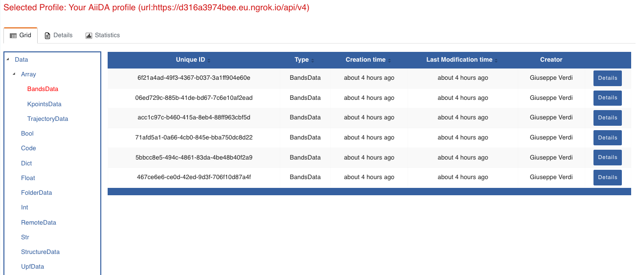
Fig. 1.3 All nodes of type BandsData, listed in the grid view.

Here we can just select one of the available nodes and click on details on the right. This will take us to the details view of that particular node:

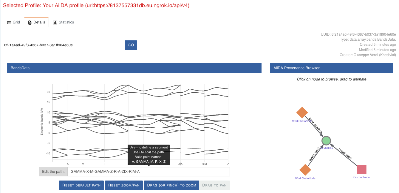
Fig. 1.4 The details view of a specific node of type BandsData.

We can see that the Explore Section can visualize the band structure stored in a BandsData node. It also shows (as it does for all types of nodes) the AiiDA Provenance Browser on its right. This tool allows us to easily explore the connections between nodes and understand, for example, how these results were obtained. For example, go to the CalcJob node that produced the band structure by finding the red square with the incoming link labeled output_band and clicking on it. This will redirect us to the details page for that CalcJob node:

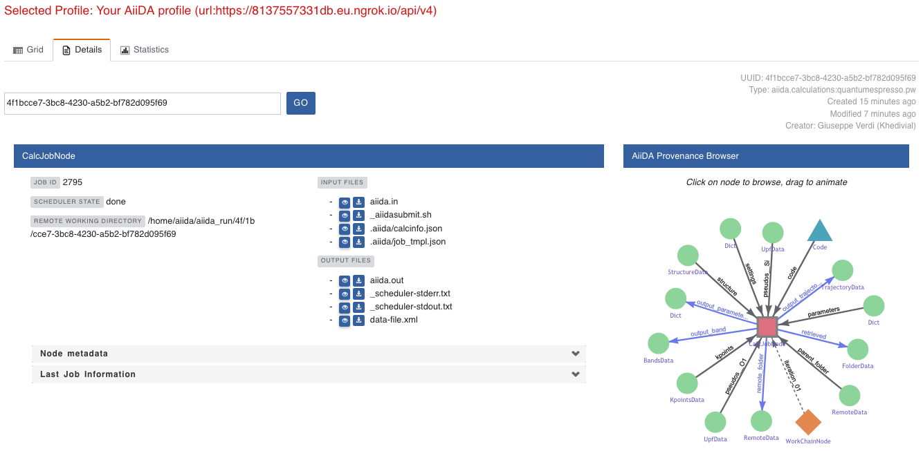
Fig. 1.5 The details view of the CalcJob node that created the original BandsData node.

You can check out here the details of the calculation, such as the input and output files, the Node metadata and Job information dropdown menus, etc. You may also want to know for which crystal structure the band structure was calculated. Although this information can also be found inside the input files, we will look for it directly in the input nodes, again by using the AiiDA Provenance Browser. This time we will look for the StructureData node (green circle) that has an outgoing link (so, the arrow points from the data node to the central current process node) with the label structure and click on it:

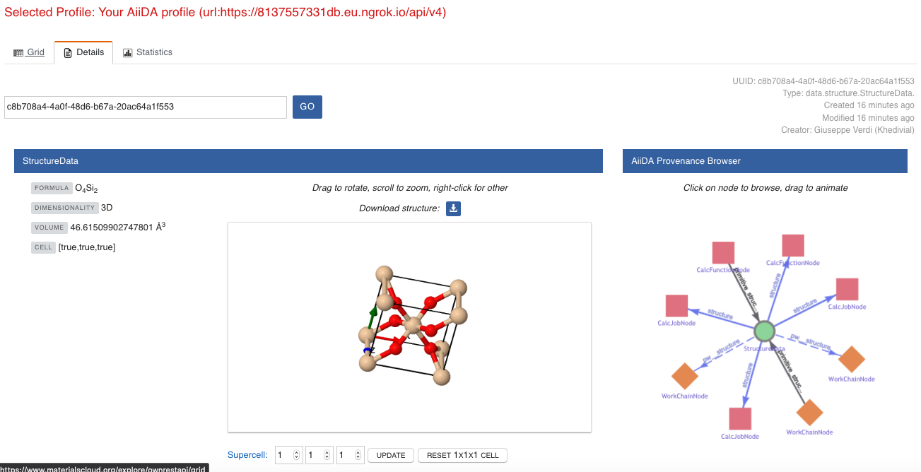
Fig. 1.6 The details view of the StructureData node that corresponds to the original BandsData node.

We can see in this particular case that the original BandsData corresponds to a Silica structure (your final structure might be different). You can look at the structure here, explore the details of the cell, etc.

Exercise: By now it is likely that your workflow has finished running. Repeat the same procedure described above to find the structure used to calculate the resulting band structure. You can identify this band structure easily as it will be the one with the newest creation time. Once you do:

1. Go to the details view for that BandsData node.

2. Look in the provenance browser for the calculation that created these bands and click on it.

3. Verify that this calculation is of type PwCalculation (look for the process_label in the node metadata subsection).

4. Look in the provenance browser for the StructureData that was used as input for this calculation.

As you can see, the explore tool of the Materials Cloud offers a very natural and intuitive interface to use for a light exploration of a database. However, you might already imagine that doing a more intensive kind of data mining of specific results this way can quickly become tedious. For this use cases, AiiDA has a more versatile tool: the QueryBuilder. This will be discussed in the section on Working with data.

1.6. Finishing the work chain

Let’s stop the REST API using Ctrl+C and close its terminal, as well as stop ngrok (also using Ctrl+C) if you are running on the AiiDAlab cluster. Use verdi process show <PK> to inspect the PwBandsWorkChain and find the PK of its band_structure output. Instead of relying on the explore tool, we can also plot the band structure using the verdi shell:

$ verdi data bands export --format mpl_pdf --output band_structure.pdf <PK>

Use the evince command or the JupyterHub file manager to open the band_structure.pdf file. It should look similar to the one shown here:

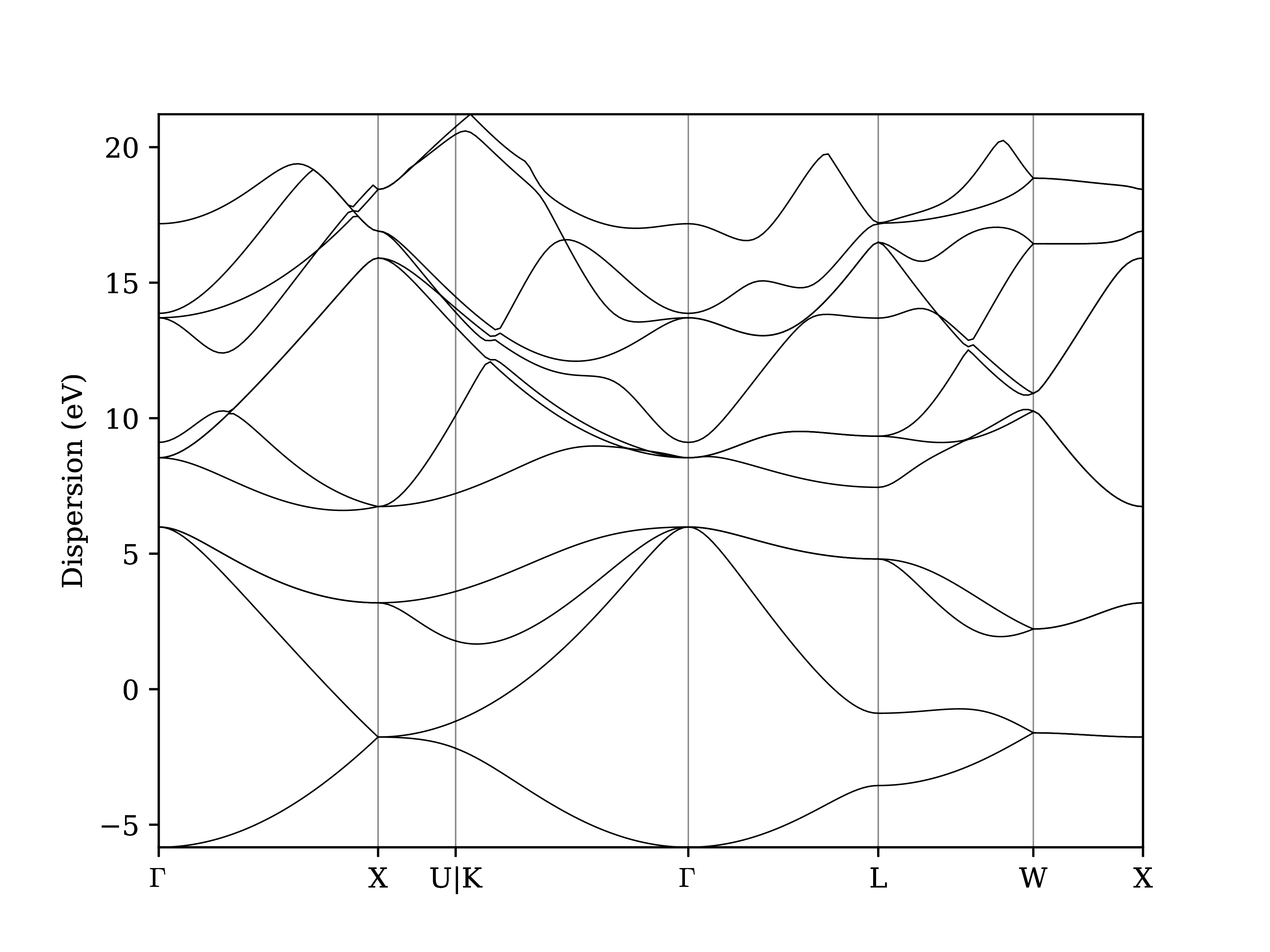
Fig. 1.7 Band structure computed by the PwBandsWorkChain.

Finally, the verdi process status command prints a hierarchical overview of the processes called by the work chain:

$ verdi process status <PK>
PwBandsWorkChain<113> Finished [0] [7:results]
    ├── PwRelaxWorkChain<115> Finished [0] [3:results]
    │   ├── PwBaseWorkChain<118> Finished [0] [7:results]
    │   │   ├── create_kpoints_from_distance<119> Finished [0]
    │   │   └── PwCalculation<123> Finished [0]
    │   └── PwBaseWorkChain<132> Finished [0] [7:results]
    │       ├── create_kpoints_from_distance<133> Finished [0]
    │       └── PwCalculation<137> Finished [0]
    ├── seekpath_structure_analysis<144> Finished [0]
    ├── PwBaseWorkChain<151> Finished [0] [7:results]
    │   ├── create_kpoints_from_distance<152> Finished [0]
    │   └── PwCalculation<156> Finished [0]
    └── PwBaseWorkChain<164> Finished [0] [7:results]
        └── PwCalculation<167> Finished [0]

The bracket [7:result] indicates the current step in the outline of the PwBandsWorkChain (step 7, with name result). The process status is particularly useful for debugging complex work chains, since it helps pinpoint where a problem occurred.

Congratulations on finishing the first part of the tutorial! In the next section, we’ll look at how to organize and query your data.