2. Working with data and querying your results
In this section of the tutorial, we will focus on how to organise and explore the data in an AiiDA database. We will use a previously created database for this tutorial. To follow the tutorial, you first need to import that archive into your database:
$ verdi import https://object.cscs.ch/v1/AUTH_b1d80408b3d340db9f03d373bbde5c1e/marvel-vms/tutorials/aiida_tutorial_2020_07_perovskites_v0.9.aiida
The import can take several minutes.
2.1. How to group nodes
AiiDA’s database is great for automatically storing all your data, but sometimes it can be tricky to navigate this flat data store. To create some order in this mass of data, you can group sets of nodes together, just as you would with files in folders on your filesystem. Each group can hold any amount of nodes and any node can be contained in any number of groups. A typical use case is to store all nodes that share a common property in a single group.
2.1.1. Listing existing groups
Lets explore the groups already present in the imported archive:
$ verdi group list -a -A
PK    Label            Type string    User
----  ---------------  -------------  ---------------
   1  tutorial_pbesol  core           aiida@localhost
   2  tutorial_lda     core           aiida@localhost
   3  tutorial_pbe     core           aiida@localhost
   4  GBRV_pbe         core.upf       aiida@localhost
   5  GBRV_pbesol      core.upf       aiida@localhost
   6  GBRV_lda         core.upf       aiida@localhost
   7  20200705-071658  core.import    aiida@localhost
The default table shows us four pieces of information:
- PK
The Primary Key of the group
- Label
The label by which the group has been named
- Type string
This tells us what “sub-class” of group this is. Type strings can be used to class certain types of data, for example here we have general groups (
core), groups containing pseudopotentials (core.upf), and an auto-generated group containing the nodes we imported from the archive (core.import). For advanced use, you can create your own group subclass plugins, with specialised methods.- User
The email of the user that created this group.
Tip
The -a and -A flags we used above ensure that groups for all type strings and users are shown respectively.
We can then inspect the content of a group by its label (if it is unique) or the PK:
$ verdi group show tutorial_pbesol
-----------------  ----------------
Group label        tutorial_pbesol
Group type_string  core
Group description  <no description>
-----------------  ----------------
# Nodes:
PK    Type         Created
----  -----------  -----------------
 380  CalcJobNode  2078D:17h:46m ago
1273  CalcJobNode  2078D:18h:03m ago
...
Conversely, if you want to see all the groups a node belongs to, you can run:
$ verdi group list -a -A --node 380
PK    Label            Type string    User
----  ---------------  -------------  ---------------
   1  tutorial_pbesol  core           aiida@localhost
   7  20200705-071658  core.import    aiida@localhost
2.1.2. Creating and manipulating groups
Lets make a new group:
$ verdi group create a_group
Success: Group created with PK = 8 and name 'a_group'
If we want to change the name of the group at any time:
$ verdi group relabel a_group my_group
Success: Label changed to my_group
Now we can add one or more nodes to it:
$ verdi group add-nodes -G my_group 380 1273
Do you really want to add 2 nodes to Group<my_group>? [y/N]: y
We can also copy the nodes from an existing group to another group:
$ verdi group copy tutorial_pbesol my_group
Warning: Destination group<my_group> already exists and is not empty.
Do you wish to continue anyway? [y/N]: y
Success: Nodes copied from group<tutorial_pbesol> to group<my_group>
$ verdi group show my_group
-----------------  ----------------
Group label        my_group
Group type_string  core
Group description  <no description>
-----------------  ----------------
# Nodes:
PK    Type         Created
----  -----------  -----------------
74  CalcJobNode  2078D:17h:51m ago
76  CalcJobNode  2078D:17h:57m ago
...
To remove nodes from the group run:
$ verdi group remove-nodes -G my_group 74
Do you really want to remove 1 nodes from Group<my_group>? [y/N]: y
and finally to remove the group entirely:
$ verdi group delete my_group
Are you sure to delete Group<my_group>? [y/N]: y
Success: Group<my_group> deleted.
Important
Any deletion operation related to groups won’t affect the nodes themselves. For example if you delete a group, the nodes that belonged to the group will remain in the database. The same happens if you remove nodes from the group – they will remain in the database but won’t belong to the group any more.
2.2. Organising groups in hierarchies
Earlier, we mentioned that groups are like files in folders on your filesystem.
As with folders and sub-folders then, as the amount of groups we have grows, we may also wish to structure our groups in a hierarchy.
Groups in AiiDA are inherently “flat”, in that groups may only contain nodes and not other groups.
However it is possible to construct virtual group hierarchies based on delimited group labels, using the grouppath utility.
Like folder paths grouppath requires delimitation by / (forward slash) characters.
Lets copy and rename the three tutorial groups:
$ verdi group copy tutorial_lda tutorial/lda/basic
$ verdi group copy tutorial_pbe tutorial/gga/pbe
$ verdi group copy tutorial_pbesol tutorial/gga/pbesol
We can now list the groups in a new way:
$ verdi group path ls -l
Path             Sub-Groups
---------------  ------------
tutorial                    3
tutorial_lda                0
tutorial_pbe                0
tutorial_pbesol             0
Note
In the terminal, paths that contain nodes are listed in bold
You can see that the actual groups that we create do not show, only the initial part of the “path”, and how many sub-groups that path contains. We can then step into a path:
$ verdi group path ls -l tutorial
Path          Sub-Groups
------------  ------------
tutorial/gga             2
tutorial/lda             1
This feature is also particularly useful in the verdi shell:
In [1]: from aiida.tools.groups import GroupPath
In [2]: for subpath in GroupPath("tutorial/gga").walk(return_virtual=False):
   ...:     print(subpath.get_group())
   ...:
"tutorial/gga/pbesol" [type core], of user aiida@localhost
"tutorial/gga/pbe" [type core], of user aiida@localhost
See also
Please see the corresponding section in the documentation for more details on groups and how to use them.
Before we continue, let us delete these paths:
$ verdi group delete  -f tutorial/lda/basic
$ verdi group delete  -f tutorial/gga/pbe
$ verdi group delete  -f tutorial/gga/pbesol
2.3. Querying the database
As you will use AiiDA to run your calculations, the database that stores all the data and the provenance will quickly grow to be very large.
To help you find the needle that you might be looking for in this big haystack, we need an efficient search tool.
AiiDA provides a tool to do exactly this: the QueryBuilder.
The QueryBuilder acts as the gatekeeper to your database, to whom you can ask questions about its contents (also referred to as queries), by specifying what are looking for.
In this final part of the tutorial, we will show an short demo on how to use the QueryBuilder to make these queries and understand/use the results.
Let’s have another look at the groups we’ve imported from the archive above, using the -C option so we also get a count of the number of nodes:
$ verdi group list --count
Info: to show groups of all types, use the `-a/--all` option.
  PK  Label            Type string    User               Node count
----  ---------------  -------------  ---------------  ------------
   5  tutorial_pbesol  core           aiida@localhost            57
   6  tutorial_lda     core           aiida@localhost            57
   7  tutorial_pbe     core           aiida@localhost            57
Each group contains a different set of 57 PwCalculation nodes (one for every different perovskite structure), organized according to the functional which was used in the calculation (LDA, PBE and PBEsol) .
Imagine you want to use this data to understand the influence of the functional on the magnetization of the structure.
Let’s build a query that helps us investigate this question.
Start the verdi shell, and load the StructureData and PwCalculation classes:
In [1]: StructureData = DataFactory('structure')
   ...: PwCalculation = CalculationFactory('quantumespresso.pw')
We start every query by creating an instance of the QueryBuilder class:
In [2]: qb = QueryBuilder()
To build a query, we append entities (nodes, groups, …) to the query.
Let’s build the query for one of the groups - say, tutorial_pbesol - step by step to help understand the process.
We first append the Group to our QueryBuilder instance:
In [3]: qb.append(Group, filters={'label': 'tutorial_pbesol'}, tag='group');
Let’s explain the different arguments used in this call of the append() method:
The first positional argument is the
Groupclass, preloaded in theverdi shell.The first keyword argument is
filters, here we filter for the group withlabelequal totutorial_pbesol.The second keyword argument is
tag. This is a reference we will use to indicate relationships between nodes in futureappend()calls (as seen below).
Next, we’ll look for all the PwCalculations in this group:
In [4]: qb.append(PwCalculation, with_group='group', tag='pw');
Here, we use the 'group' tag we created in the previous step to query for PwCalculation’s in the tutorial_pbesol group using the with_group relationship argument.
Moreover, we once again tag this append step of our query with pw.
Let’s have a look at how many PwCalculation nodes we have in the tutorial_pbesol group:
In [5]: qb.count()
Out[5]: 57
Great, now let’s figure out which structures are magnetic!
Of course, the information we are interested in are the structures and their absolute magnetization, which we’ll query for in the final two steps.
First, we’ll append the StructureData to the query:
In [6]: qb.append(StructureData, with_outgoing='pw', project='extras.formula');
In this step, we’ve used the with_outgoing relationship to look for structures that have an outgoing link to the PwCalculations referenced with the pw tag.
That means that from the PwCalculation’s perspective, the StructureData is an input.
We also use the project keyword argument to project the formula of the structure, which has been conveniently stored in the extras of these StructureData nodes for the purpose of this tutorial.
By projecting the formula, it will be a part of the results of our query.
Try looking at the results of the current query using qb.all():
In [7]: qb.all()
The final append() call puts using relationships, filters and projections together.
Here we are looking for the output_parameters Dict nodes, which are outputs of the PwCalculation nodes.
However, we are only interested in structures for which the absolute_magnetization is larger than zero:
In [8]: qb.append(
   ...:     Dict, with_incoming='pw', filters={'attributes.absolute_magnetization': {'>': 0.0}},
   ...:     project='attributes.absolute_magnetization'
   ...: );
Let’s go over the arguments again:
The first positional argument tells the
QueryBuilderwe want to appendDictnodes to our query.
with_incomingindicates there is an incoming link from aPwCalculation, referenced by the'pw'tag.We’re
filter-ing for magnetic structures, i.e. withabsolute_magnetizationabove zero.Finally, we
projectthe absolute magnetization so it is added to the list of our results for each query result.
Our query is now complete! Let’s have a look at the results:
In [9]: qb.all()
Out[9]:
[['LaMnO3', 3.5],
 ['MnO3Sr', 3.15],
 ['CoO3Sr', 2.42],
 ['FeLaO3', 3.11],
 ['CoLaO3', 1.13],
 ['NiO3Sr', 0.77],
 ['FeO3Sr', 3.38]]
You can see that we’ve found 7 magnetic structures for the calculations in the tutorial_pbesol group, along with their formulas and magnetizations.
We’ve set up a script (demo_query.py) that performs a similar query to obtain the magnetization and smearing energy for all results in the three groups, and then postprocess the data to visualize it.
You can find it in the dropdown panel below:
Query demo script
from IPython.display import Image
from datetime import datetime, timedelta
import numpy as np
from matplotlib import gridspec, pyplot as plt

PwCalculation = CalculationFactory('quantumespresso.pw')
StructureData = DataFactory('structure')
KpointsData = DataFactory('array.kpoints')
Dict = DataFactory('dict')
UpfData = DataFactory('upf')


def plot_results(query_res):
    """
    :param query_res: The result of an instance of the QueryBuilder
    """
    smearing_unit_set, magnetization_unit_set, pseudo_family_set = set(), set(
    ), set()
    # Storing results:
    results_dict = {}
    for pseudo_family, formula, smearing, smearing_units, mag, mag_units in query_res:
        if formula not in results_dict:
            results_dict[formula] = {}
        # Storing the results:
        results_dict[formula][pseudo_family] = (smearing, mag)
        # Adding to the unit set:
        smearing_unit_set.add(smearing_units)
        magnetization_unit_set.add(mag_units)
        pseudo_family_set.add(pseudo_family)

    # Sorting by formula:
    sorted_results = sorted(results_dict.items())
    formula_list = next(zip(*sorted_results))
    nr_of_results = len(formula_list)

    # Checks that I have not more than 3 pseudo families.
    # If more are needed, define more colors
    #pseudo_list = list(pseudo_family_set)
    if len(pseudo_family_set) > 3:
        raise Exception('I was expecting 3 or less pseudo families')

    colors = ['b', 'r', 'g']

    # Plotting:
    plt.clf()
    fig = plt.figure(figsize=(16, 9), facecolor='w', edgecolor=None)
    gs = gridspec.GridSpec(2, 1, hspace=0.01, left=0.1, right=0.94)

    # Defining barwidth
    barwidth = 1. / (len(pseudo_family_set) + 1)
    offset = [
        -0.5 + (0.5 + n) * barwidth for n in range(len(pseudo_family_set))
    ]
    # Axing labels with units:
    yaxis = ("Smearing energy [{}]".format(smearing_unit_set.pop()),
             "Total magnetization [{}]".format(magnetization_unit_set.pop()))
    # If more than one unit was specified, I will exit:
    if smearing_unit_set:
        raise ValueError('Found different units for smearing')
    if magnetization_unit_set:
        raise ValueError('Found different units for magnetization')

    # Making two plots, the top one for the smearing, the bottom one for the magnetization
    for index in range(2):
        ax = fig.add_subplot(gs[index])
        for i, pseudo_family in enumerate(pseudo_family_set):
            X = np.arange(nr_of_results) + offset[i]
            Y = np.array([
                thisres[1][pseudo_family][index] for thisres in sorted_results
            ])
            ax.bar(X,
                   Y,
                   width=0.2,
                   facecolor=colors[i],
                   edgecolor=colors[i],
                   label=pseudo_family)
        ax.set_ylabel(yaxis[index], fontsize=14, labelpad=15 * index + 5)
        ax.set_xlim(-0.5, nr_of_results - 0.5)
        ax.set_xticks(np.arange(nr_of_results))
        if index == 0:
            plt.setp(ax.get_yticklabels()[0], visible=False)
            ax.xaxis.tick_top()
            ax.legend(loc=3, prop={'size': 18})
        else:
            plt.setp(ax.get_yticklabels()[-1], visible=False)
        for i in range(0, nr_of_results, 2):
            ax.axvspan(i - 0.5, i + 0.5, facecolor='y', alpha=0.2)
        ax.set_xticklabels(list(formula_list),
                           rotation=90,
                           size=14,
                           ha='center')
    plt.savefig('demo_query.pdf')


qb = QueryBuilder().append(
    Group,
    filters={
        'label': {
            'like': 'tutorial_%'
        }
    },
    project='label',
    tag='group').append(PwCalculation, tag='calculation',
                        with_group='group').append(
                            StructureData,
                            project=['extras.formula'],
                            tag='structure',
                            with_outgoing='calculation').append(
                                Dict,
                                tag='results',
                                project=[
                                    'attributes.energy_smearing',
                                    'attributes.energy_smearing_units',
                                    'attributes.total_magnetization',
                                    'attributes.total_magnetization_units',
                                ],
                                with_incoming='calculation')

plot_results(qb.all())
Download it using wget:
$ wget https://aiida-tutorials.readthedocs.io/en/tutorial-2020-bigmap-lab/_downloads/6773ba4cad0c046e468d13e15186cdd8/demo_query.py
and use verdi run to execute it:
$ verdi run demo_query.py
The resulting plot should look like the one shown in Fig. 2.1.
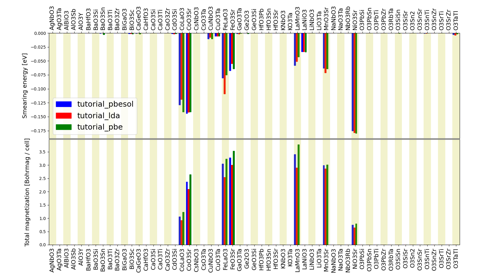
Fig. 2.1 Comparison of the absolute magnetization and smearing energy of the cell of the perovskite structures, calculated with different functionals.
2.4. What next?
You now have a first taste of the type of problems AiiDA tries to solve. Here are some options for how to continue:
Get a more detailed view of how to manipulate AiiDA objects in the extra section of this tutorial.
Register for the in-depth tutorial organised July 5-9 2021.
Try setting up AiiDA directly on your laptop.